Distribution Layers

Distribution Layers#

import numpy as np
import matplotlib.pyplot as plt
from scipy import stats
from scipy.integrate import quad
from progressbar import progressbar as pbar
from rlxutils import subplots, copy_func
import seaborn as sns
import pandas as pd 

import tensorflow as tf
import tensorflow_probability as tfp
tfd = tfp.distributions
tfb = tfp.bijectors

%matplotlib inline

2022-03-08 06:24:42.627938: W tensorflow/stream_executor/platform/default/dso_loader.cc:64] Could not load dynamic library 'libcudart.so.11.0'; dlerror: libcudart.so.11.0: cannot open shared object file: No such file or directory
2022-03-08 06:24:42.627973: I tensorflow/stream_executor/cuda/cudart_stub.cc:29] Ignore above cudart dlerror if you do not have a GPU set up on your machine.

The output of a distribution layer is a distribution#

In distribution layers:

the input are regular tensors
the output are distributions objects that are use the input tensors as parameters
the event_shape is the number of dimensions
each dimension will be modelled by an independent Normal distribution \(\mathcal{N}(\mu, \sigma)\)
each independent normal is governed by two parameters

for instance, a 2D independent normal distribution with

\[(x,y) \sim \mathcal{N}_x(-10, 5) \times \mathcal{N}_y(20, 8)\]

inormal_layer = tfp.layers.IndependentNormal(event_shape=1)

inormal_layer.get_config()

{'name': 'independent_normal_2',
 'trainable': True,
 'dtype': 'float32',
 'function': ('4wAAAAAAAAAAAAAAAAcAAAAEAAAAHwAAAHOmAAAAiAF8AGkAfAGkAY4BfQJ0AHwCagF0AmoDgwJ9\nA3wDciyHAGYBZAFkAoQIbgKIAH0EdARqBXwCfARkA40CfQV8BaAGoQB9BnwFfAZfB3wDco58BmQE\nGQBqCHwGXwh8BmQEGQBqCXwGXwl8BmQEGQBqAXwGXwF8BmQEGQBqCHwFXwp8BmQEGQBqCXwFXwlu\nEHwGagh8BV8KfAZqCXwFXwl8BXwGZgJTACkF+kRXcmFwcyBgbWFrZV9kaXN0cmlidXRpb25fZm5g\nIHRvIHJldHVybiBib3RoIGRpc3QgYW5kIGNvbmNyZXRlIHZhbHVlLmMBAAAAAAAAAAAAAAABAAAA\nBAAAABMAAABzDgAAAHQAoAGIAHwAgwGhAVMAqQFOKQLaDHRlbnNvcl90dXBsZdoLVGVuc29yVHVw\nbGUpAdoBZKkB2hRjb252ZXJ0X3RvX3RlbnNvcl9mbqkA+m0vb3B0L2FuYWNvbmRhL2VudnMvcDM5\nL2xpYi9weXRob24zLjkvc2l0ZS1wYWNrYWdlcy90ZW5zb3JmbG93X3Byb2JhYmlsaXR5L3B5dGhv\nbi9sYXllcnMvZGlzdHJpYnV0aW9uX2xheWVyLnB52gg8bGFtYmRhPqkAAADzAAAAAHo6RGlzdHJp\nYnV0aW9uTGFtYmRhLl9faW5pdF9fLjxsb2NhbHM+Ll9mbi48bG9jYWxzPi48bGFtYmRhPikC2gxk\naXN0cmlidXRpb25yBwAAAOn/////KQvaCmlzaW5zdGFuY2XaBWR0eXBl2gtjb2xsZWN0aW9uc9oI\nU2VxdWVuY2XaA2R0Y9oQX1RlbnNvckNvZXJjaWJsZdoGX3ZhbHVl2hFfdGZwX2Rpc3RyaWJ1dGlv\nbtoFc2hhcGXaCWdldF9zaGFwZdoGX3NoYXBlKQdaBWZhcmdzWgdma3dhcmdzcgUAAABaDHZhbHVl\nX2lzX3NlcVokbWF5YmVfY29tcG9zaXRlX2NvbnZlcnRfdG9fdGVuc29yX2ZucgwAAADaBXZhbHVl\nqQJyBwAAANoUbWFrZV9kaXN0cmlidXRpb25fZm5yCAAAAHIJAAAA2gNfZm6kAAAAcyoAAAAAAg4B\nDgMC/w4BAv4CAwQBAgEC/gYJCAQGBAQBDAEMAQwBDAEOAggBCAE=\n',
  None,
  (<function tensorflow_probability.python.distributions.distribution.Distribution.sample(self, sample_shape=(), seed=None, name='sample', **kwargs)>,
   <function tensorflow_probability.python.layers.distribution_layer.IndependentNormal.__init__.<locals>.<lambda>(t)>)),
 'function_type': 'lambda',
 'module': 'tensorflow_probability.python.layers.distribution_layer',
 'output_shape': None,
 'output_shape_type': 'raw',
 'output_shape_module': None,
 'arguments': {},
 'make_distribution_fn': 'gAWVkQMAAAAAAACMF2Nsb3VkcGlja2xlLmNsb3VkcGlja2xllIwNX2J1aWx0aW5fdHlwZZSTlIwK\nTGFtYmRhVHlwZZSFlFKUKGgCjAhDb2RlVHlwZZSFlFKUKEsBSwBLAEsBSwVLE0MOdACgAXwAiACI\nAaEDUwCUToWUjBFJbmRlcGVuZGVudE5vcm1hbJSMA25ld5SGlIwBdJSFlIxtL29wdC9hbmFjb25k\nYS9lbnZzL3AzOS9saWIvcHl0aG9uMy45L3NpdGUtcGFja2FnZXMvdGVuc29yZmxvd19wcm9iYWJp\nbGl0eS9weXRob24vbGF5ZXJzL2Rpc3RyaWJ1dGlvbl9sYXllci5weZSMCDxsYW1iZGE+lE24A0MA\nlIwLZXZlbnRfc2hhcGWUjA12YWxpZGF0ZV9hcmdzlIaUKXSUUpR9lCiMC19fcGFja2FnZV9flIwk\ndGVuc29yZmxvd19wcm9iYWJpbGl0eS5weXRob24ubGF5ZXJzlIwIX19uYW1lX1+UjDd0ZW5zb3Jm\nbG93X3Byb2JhYmlsaXR5LnB5dGhvbi5sYXllcnMuZGlzdHJpYnV0aW9uX2xheWVylIwIX19maWxl\nX1+UjG0vb3B0L2FuYWNvbmRhL2VudnMvcDM5L2xpYi9weXRob24zLjkvc2l0ZS1wYWNrYWdlcy90\nZW5zb3JmbG93X3Byb2JhYmlsaXR5L3B5dGhvbi9sYXllcnMvZGlzdHJpYnV0aW9uX2xheWVyLnB5\nlHVOTmgAjBBfbWFrZV9lbXB0eV9jZWxslJOUKVKUaCApUpSGlHSUUpSMHGNsb3VkcGlja2xlLmNs\nb3VkcGlja2xlX2Zhc3SUjBJfZnVuY3Rpb25fc2V0c3RhdGWUk5RoJX2UfZQoaBtoEYwMX19xdWFs\nbmFtZV9flIwsSW5kZXBlbmRlbnROb3JtYWwuX19pbml0X18uPGxvY2Fscz4uPGxhbWJkYT6UjA9f\nX2Fubm90YXRpb25zX1+UfZSMDl9fa3dkZWZhdWx0c19flE6MDF9fZGVmYXVsdHNfX5ROjApfX21v\nZHVsZV9flGgcjAdfX2RvY19flE6MC19fY2xvc3VyZV9flGgAjApfbWFrZV9jZWxslJOUSwGFlFKU\naDWJhZRSlIaUjBdfY2xvdWRwaWNrbGVfc3VibW9kdWxlc5RdlIwLX19nbG9iYWxzX1+UfZRoC2gc\naAuTlHN1hpSGUjAu\n',
 'convert_to_tensor_fn': 'sample',
 'event_shape': 1,
 'validate_args': False}

calling the layer with some input data produces a distribution object PARAMETRIZED BY THE INPUT DATA

you get a distribution for each row (or elements in dimension 0) of the input data.

input_x = np.random.randint(5, size=(2,2))*1.+5

print(input_x)
output_distribution = inormal_layer(input_x)
type(output_distribution)

[[8. 9.]
 [9. 6.]]

2022-03-08 06:27:38.111928: W tensorflow/stream_executor/platform/default/dso_loader.cc:64] Could not load dynamic library 'libcuda.so.1'; dlerror: libcuda.so.1: cannot open shared object file: No such file or directory
2022-03-08 06:27:38.111977: W tensorflow/stream_executor/cuda/cuda_driver.cc:269] failed call to cuInit: UNKNOWN ERROR (303)
2022-03-08 06:27:38.112010: I tensorflow/stream_executor/cuda/cuda_diagnostics.cc:156] kernel driver does not appear to be running on this host (rlxyoga): /proc/driver/nvidia/version does not exist
2022-03-08 06:27:38.113438: I tensorflow/core/platform/cpu_feature_guard.cc:151] This TensorFlow binary is optimized with oneAPI Deep Neural Network Library (oneDNN) to use the following CPU instructions in performance-critical operations:  AVX2 FMA
To enable them in other operations, rebuild TensorFlow with the appropriate compiler flags.
2022-03-08 06:27:38.158592: W tensorflow/python/util/util.cc:368] Sets are not currently considered sequences, but this may change in the future, so consider avoiding using them.

tensorflow_probability.python.layers.internal.distribution_tensor_coercible._TensorCoercible

output_distribution.batch_shape

TensorShape([2])

# which we can use as any distribution object
s = output_distribution.sample(1000).numpy()
s.shape

(1000, 2, 1)

print ("means", np.mean(s, axis=0)[:,0])
print ("stds ", np.std(s, axis=0)[:,0])

means [8.07702  8.886362]
stds  [9.426311 6.080694]

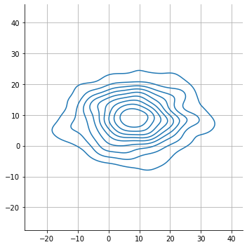
ev = 0
sns.displot(
    x = s[:,0,ev],
    y = s[:,1,ev],
    kind="kde", rug=False
)
plt.axis("equal")
plt.grid();

../_images/dc7fda1ef738fda929e70a7b3d56d4043628e558c8c5d750de185e36206c4ea3.png

the batch size fo the distribution is determined by the input data shape.

the last dimension of the input data must match the number of parameters required by the distribution
the remaining dimensions determine the distributions batch_shape

input_x = np.random.randint(5, size=(2,3,4,2))*1.+5
print(input_x)
output_distribution = inormal_layer(input_x)
output_distribution.batch_shape

[[[[5. 7.]
   [6. 8.]
   [8. 5.]
   [9. 5.]]

  [[6. 6.]
   [9. 6.]
   [6. 6.]
   [7. 7.]]

  [[9. 9.]
   [6. 8.]
   [9. 8.]
   [5. 8.]]]


 [[[9. 8.]
   [7. 8.]
   [6. 8.]
   [9. 9.]]

  [[5. 5.]
   [8. 8.]
   [5. 7.]
   [9. 6.]]

  [[6. 9.]
   [6. 7.]
   [6. 8.]
   [6. 7.]]]]

TensorShape([2, 3, 4])

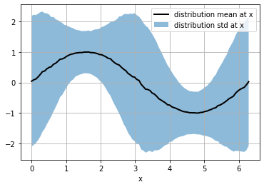
observe how continuous input data can parametrize a continuum of distributions

x = np.linspace(0,2*np.pi,100)
input_x = np.vstack([np.sin(x), 1+np.cos(x*2)]).T
input_x.shape

(100, 2)

output_distribution = inormal_layer(input_x)
output_distribution.batch_shape

TensorShape([100])

s = output_distribution.sample(10000).numpy()[:,:,0]
s.shape

(10000, 100)

so, for each x we have a different distribution (with different mean and std) and we have a sample of 10K elements of each distribution

smean = np.mean(s, axis=0)
sstd  = np.std(s, axis=0)

plt.plot(x, smean, color="black", lw=2, label="distribution mean at x")
plt.fill_between(x, smean-sstd, smean+sstd, alpha=.5, label="distribution std at x")
plt.grid(); plt.legend(); plt.xlabel("x")

Text(0.5, 0, 'x')

../_images/a5f83e498e3e1ae2b8a6ccde76b592fcbbbd264b99e610211e6eaaef99288faa.png

the probability of the output_distribution is the probability for each distribution in the generated batch.

\[\texttt{distribution.log_prob(x)}= \sum_d \sum_k \log P_d(x_k) \; \; \; \forall x_k \in \mathbf{x}\text{ and each distribution }d\text{ in the batch}\]

and \(\mathbf{x}\) must comply with the batch_size of the distribution batch,

note the difference between

input_x, which is the input data to the distribution layer and produces a distribution (a batch of distributions)
x, which is the data to which we compute probabilities using the output of the distribution layer.

# some example points
input_x = np.r_[[[10.,1.],[11.,2.], [12.,3.]]]
output_distribution = inormal_layer(input_x)
output_distribution.batch_shape

TensorShape([3])

x = np.linspace(10,12,6)
print (x)
output_distribution.log_prob(x)

[10.  10.4 10.8 11.2 11.6 12. ]

<tf.Tensor: shape=(3,), dtype=float32, numpy=array([ -9.699949, -10.351176, -12.675131], dtype=float32)>

# create a scipy.stats distribution for each input_x
distrs = [stats.norm(*i) for i in input_x]

[np.sum(np.log(i.pdf(x))) for i in distrs]

[-9.913631199228035, -10.022514282587707, -12.594193820125582]

Distribution layer in a Keras model#

the previous layer MUST provide the shape of the parameters required by the distribution layer.

Either from an input layer directly.

input_x = np.random.randint(5, size=(3,2))*1.+5
print (input_x)

inp  = tf.keras.layers.Input(shape=(2,))
out  = tfp.layers.IndependentNormal(1)(inp)

m    = tf.keras.models.Model(inp, out)

[[5. 9.]
 [5. 9.]
 [8. 7.]]

moutput = m(input_x)
moutput

<tfp.distributions._TensorCoercible 'tensor_coercible' batch_shape=[3] event_shape=[1] dtype=float32>

s = moutput.sample(10000).numpy()[:,:,0]
s.shape

(10000, 3)

print ("means", np.mean(s, axis=0))
print ("stds ", np.std(s, axis=0))

means [5.0123467 5.0472274 8.039777 ]
stds  [8.997255  8.847788  7.1187677]

The .predict of a model with a distribution layer output is a sample (by default)

m.predict(input_x)

array([[-3.8559008],
       [19.388023 ],
       [ 5.0254173]], dtype=float32)

We can, of course, use other layers previous to the distribution layer and the input_x is transformed accordingly

and everything is learnable.

input_x = np.random.random(size=(3,5))+.1
print (input_x)

inp  = tf.keras.layers.Input(shape=(5,))
den  = tf.keras.layers.Dense(2, activation="sigmoid", name="dense", bias_initializer="glorot_uniform")(inp)
out  = tfp.layers.IndependentNormal(1)(den)

m    = tf.keras.models.Model(inp, out)

[[1.009664   0.55301791 0.62143092 0.1414634  0.16226084]
 [1.09063203 0.99716617 0.61228457 0.42877567 0.14910155]
 [1.05257904 0.90082675 0.26170321 0.35503394 0.77613307]]

moutput = m(input_x)
moutput

<tfp.distributions._TensorCoercible 'tensor_coercible' batch_shape=[3] event_shape=[1] dtype=float32>

s = moutput.sample(100000).numpy()[:,:,0]
s.shape

(100000, 3)

the sample means and stds correspond to the transformed input_x according to the intermediate dense layer.

observe that in this setting, the IndependantNormal layer passes the std parameter through a tf.keras.activations.softplus transformation to ensure the standard deviation is \(>0\)

print ("means", np.mean(s, axis=0))
print ("stds ", np.std(s, axis=0))

means [0.11219823 0.06530911 0.0980479 ]
stds  [1.0946325 1.1205078 1.1397614]

W, b = m.get_layer("dense").get_weights()
input_x.shape, W.shape, b.shape

((3, 5), (5, 2), (2,))

sigm = lambda x: 1/(1+np.exp(-x))
params = sigm(input_x.dot(W) +b)
params

array([[0.11328718, 0.69129696],
       [0.0637393 , 0.72553953],
       [0.10460352, 0.7521605 ]])

print ("means         ", params[:,0])
print ("softplus stds ", np.log(np.exp(params[:,1])+1))

means          [0.11328718 0.0637393  0.10460352]
softplus stds  [1.09737919 1.12032335 1.13833888]

Distribution Layers

Contents

Distribution Layers#

The output of a distribution layer is a distribution#

Distribution layer in a Keras model#