Recorridos sobre grafos
Contents
!wget -nc --no-cache -O init.py -q https://raw.githubusercontent.com/rramosp/introalgs.v1/main/content/init.py
import init; init.init(force_download=False);
Recorridos sobre grafos
Objetivo
Aprender las diferentes formas de recorrer un grafo y construir los algoritmos correspondientes.
## Preguntas básicas
¿En qué consiste el recorrido DFS sobre un grafo?
¿En qué consiste el recorrido BFS sobre un grafo?
Introducción
Al igual que en los árboles, los grafos son estructuras en las cuales una de las principales operaciones es el recorrido sobre ellas. Trataremos en este módulo las diferentes formas en que se recorren los árboles.
Recorrido DFS. Recibe este nombre porque son las iniciales de las palabras en inglés Depth First Search: búsqueda primero en profundidad. El recorrido DFS consiste en: estando ubicados en un vértice i cualquiera, determinar los vértices adyacentes, de esos vértices adyacentes elegir uno que no haya sido visitado y a partir de ahí iniciar nuevamente recorrido DFS. Observe que estamos planteando una definición recursiva para el recorrido.
Recorrido BFS. Recibe este nombre porque son las iniciales de las palabras en inglés Breadth First Search: búsqueda primero a lo ancho. Hay una diferencia sustancial entre este recorrido y el DFS: mientras que en el recorrido DFS no se visitan de una vez todos los adyacentes a un vértice dado, aquí hay que visitar primero todos los vértices adyacentes a un vértice dado antes de continuar el recorrido
Ejemplo de uso e implementación
usaremos colas para controlar y determinar un recorrido BFS o BFS. Observa el uso de deque en Python
from collections import deque
import numpy as np
x = np.random.randint(100, size=10)
print("int list  ", x)
queue = deque()
for i in x:
    queue.append(i)
print("pop       ", end=' ')
while len(queue)>0:
    print(queue.pop(), end=' ')


queue = deque()
for i in x:
    queue.append(i)
print("\npop left  ", end=' ')
while len(queue)>0:
    print(queue.popleft(), end=' ')
int list   [17  9 36 40 76 79 86 25 65 15]
pop        15 65 25 86 79 76 40 36 9 17
pop left   17 9 36 40 76 79 86 25 65 15
Recorridos sobre un laberinto
Observa cómo implemnetamos un recorrido con obstáculos:
cómo describrimos el laberinto
cómo el laberinto es equivalente a un grafo
import numpy as np
import matplotlib.pyplot as plt
import pandas as pd
%matplotlib inline
EMPTY, WALL, TARGET, USED = ".","X","T","o"
c  = pd.Series({"EMPTY": ".", "WALL":"X", "TARGET":"T", "USED":"o"})
ci = pd.Series({".": 0, "X": 255, "T":100, "o":200})

def plot_map(grid,p=[]):
    img = np.r_[[[ci[i] for i in j] for j in grid]]
    plt.imshow(img, alpha=.5)
    if(len(p)>0):
        for i in range(len(p)-1):
            plt.plot([p[i][1],p[i+1][1]],[p[i][0],p[i+1][0]], color="black", lw=4)
        plt.title("path length = %d"%len(p))

    plt.xticks(list(range(img.shape[1])), list(range(img.shape[1])))
    plt.yticks(list(range(img.shape[0])), list(range(img.shape[0])))

def possible_moves(grid, y,x):
    moves = [ [y,x+1], [y-1,x], [y,x-1], [y+1,x]]

    moves = [(my,mx) for my,mx in moves if mx>=0 and mx<len(grid[0]) and \
                                           my>=0 and my<len(grid) and grid[my][mx]!=c.WALL]
    return moves
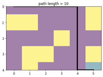
grid = ["...XX",
        "....X",
        ".X..T"]

plot_map(grid)
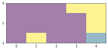
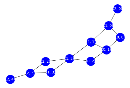
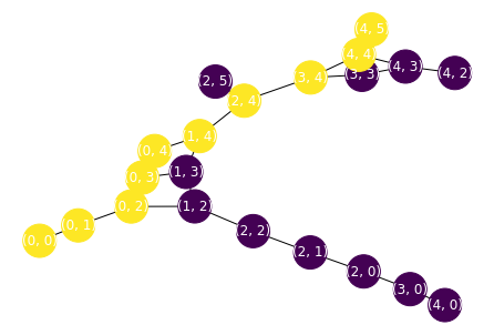
este laberinto es equivalente al siguiente grafo.
import networkx as nx
import itertools
def draw_graph(grid, path=None, node_size=900, font_color="white"):
    g = nx.Graph()
    g.add_nodes_from([(i,j) for i,j in itertools.product(list(range(len(grid))), list(range(len(grid[0])))) if grid[i][j]!="X"])
    for i,j in g.nodes:
        for ni,nj in possible_moves(grid, i,j):
            g.add_edge((i,j), (ni,nj))

    if path is None:
        c = "blue"
    else:
        c = [1 if i in p else 0 for i in g.nodes.keys()]
    nx.drawing.draw(g, with_labels=True,
                    node_alpha=.2, node_color=c,
                    node_size=node_size, font_color=font_color)
draw_graph(grid)
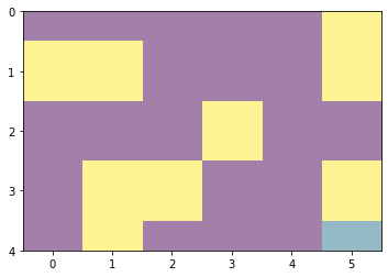
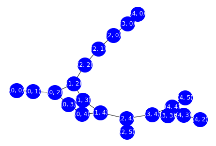
preuba con distintos laberintos para construir tu intuición del grafo asociado
grid = [".....X",
        "XX...X",
        "...X..",
        ".XX..X",
        ".X...T"]

plot_map(grid)
draw_graph(grid)
Breath First Search
This is breadth first. We put the initial node into the queue. Then repeat this procedure until visit the goal node or visit all available nodes: take the first from the queue, check if it was visited or not, check if it’s the goal, put all neighbours in the end of the queue, repeat. For each step we track not only the nodes, but directions and the path for the current node too.
does it give the best answer?
See here.
from collections import deque

def bfs_search(grid, verbose=True):
    n_iterations   = 0
    max_queue_len  = 0
    start = (0, 0)
    queue = deque([([], start)])
    visited = set()
    while queue:
        n_iterations += 1
        max_queue_len = max_queue_len if len(queue) < max_queue_len else len(queue)
        path, (y,x) = queue.popleft()
        if grid[y][x] == c.TARGET:
            if verbose:
                print("n_iterations %d, max_queue_len %d"%(n_iterations, max_queue_len))
            return path+[(y,x)]
        if (y,x) in visited:
            continue
        visited.add((y,x))
        for move in possible_moves(grid,y,x):
            queue.append((path + [(y,x)], move))

    return []
p=bfs_search(grid)
print("success", len(p)>0)
plot_map(grid, p)
n_iterations 39, max_queue_len 8
success True
print(p)
[(0, 0), (0, 1), (0, 2), (0, 3), (0, 4), (1, 4), (2, 4), (3, 4), (4, 4), (4, 5)]
draw_graph(grid, path=p)
Depth First Search
This is depth first. We simply use the other way around.
Does it give the best answer?
How is its computational complexity as compared with BFS?
from collections import deque

def dfs_search(grid, verbose=True):
    n_iterations   = 0
    max_queue_len  = 0
    start = (0, 0)
    queue = deque([([], start)])
    visited = set()
    while queue:
        n_iterations += 1
        max_queue_len = max_queue_len if len(queue) < max_queue_len else len(queue)
        path, (y,x) = queue.pop()
        if grid[y][x] == c.TARGET:
            if verbose:
                print("n_iterations %d, max_queue_len %d"%(n_iterations, max_queue_len))
            return path+[(y,x)]
        if (y,x) in visited:
            continue
        visited.add((y,x))
        for move in possible_moves(grid,y,x):
            queue.append((path + [(y,x)], move))
    return []
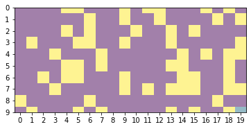
def generate_maze(size, prob=.7):
    grid = (np.random.random(size=size)>prob)*1
    grid = [[c.WALL if grid[x,y] else c.EMPTY for y in range(grid.shape[1])] for x in range(grid.shape[0])]
    grid[-1][-1]=c.TARGET
    return grid

grid = generate_maze(size=(10,20))
plot_map(grid)
print(possible_moves(grid, 1,1))
[(1, 2), (0, 1), (1, 0), (2, 1)]
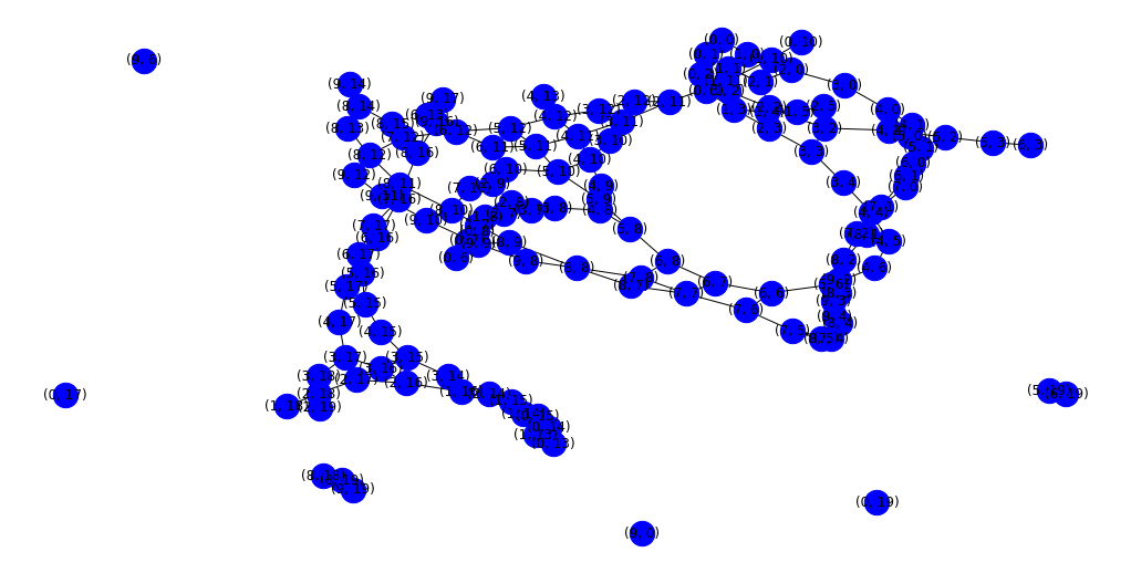
plt.figure(figsize=(14,7))
draw_graph(grid, node_size=500, font_color="black")
p=dfs_search(grid)
print("success", len(p)>0)
plot_map(grid, p)
success False

plt.figure(figsize=(14,7))
draw_graph(grid, node_size=400, font_color="black", path=p)
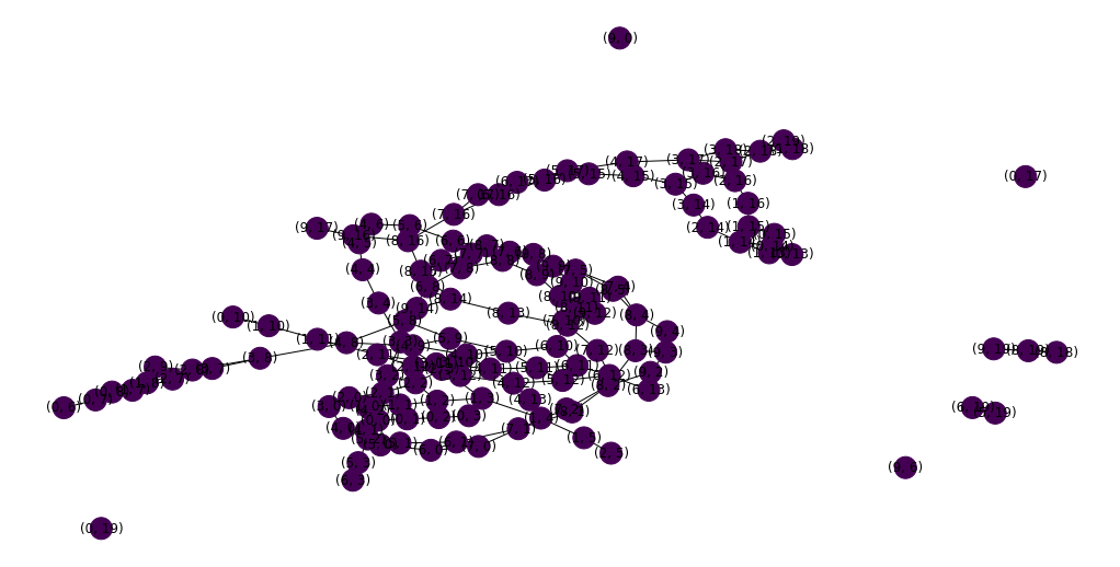
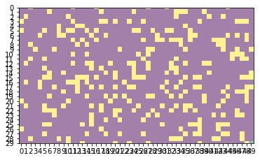
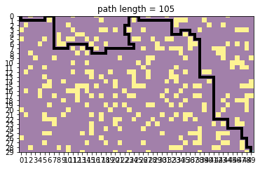
grid = generate_maze(size=(30,50), prob=.8)
plot_map(grid)
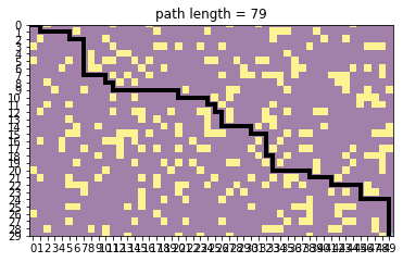
p_bfs = bfs_search(grid)
print ("success", len(p_bfs)>0)
%timeit bfs_search(grid, verbose=False)
plot_map(grid, p_bfs)
n_iterations 3890, max_queue_len 117
success True
10 loops, best of 3: 110 ms per loop
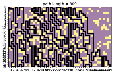
p_dfs = dfs_search(grid)
print ("success", len(p_dfs)>0)
%timeit dfs_search(grid, verbose=False)
plot_map(grid, p_dfs)
n_iterations 1868, max_queue_len 1125
success True
10 loops, best of 3: 79.9 ms per loop
let’s shorten the answer of DFS
is it now the best answer?
pp = np.r_[p_dfs]
i=0
while i<len(pp):
    for k in range(i+2, len(pp)):
        if np.sum(np.abs(pp[i]-pp[k]))==1:
            pp = np.concatenate((pp[:i+1], list(pp[k:])))
            break
    i+=1
plot_map(grid, pp)
observe computing times. larger mazes makes DFS more iterations (but slower due to data structures which should be improved)
grid = generate_maze(size=(10,20), prob=.8)
%timeit bfs_search(grid, verbose=False)
%timeit dfs_search(grid, verbose=False)

print ("bfs solution len", len(bfs_search(grid)))
print ("dfs solution len", len(dfs_search(grid)))
100 loops, best of 3: 13.5 ms per loop
100 loops, best of 3: 10.4 ms per loop
n_iterations 485, max_queue_len 59
bfs solution len 29
n_iterations 314, max_queue_len 115
dfs solution len 85
grid = generate_maze(size=(20,30))
%timeit bfs_search(grid, verbose=False)
%timeit dfs_search(grid, verbose=False)

print ("bfs solution len", len(bfs_search(grid)))
print ("dfs solution len", len(dfs_search(grid)))
10 loops, best of 3: 23.7 ms per loop
10 loops, best of 3: 23.8 ms per loop
bfs solution len 0
dfs solution len 0
grid = generate_maze(size=(50,50))
%timeit bfs_search(grid, verbose=False)
%timeit dfs_search(grid, verbose=False)

print ("bfs solution len", len(bfs_search(grid)))
print ("dfs solution len", len(dfs_search(grid)))
10 loops, best of 3: 151 ms per loop
10 loops, best of 3: 107 ms per loop
n_iterations 4901, max_queue_len 151
bfs solution len 101
n_iterations 2785, max_queue_len 785
dfs solution len 589