LAB 2.1 - Customized loss function

!wget -nc --no-cache -O init.py -q https://raw.githubusercontent.com/rramosp/2021.deeplearning/main/content/init.py
import init; init.init(force_download=False); init.get_weblink() 

from local.lib.rlxmoocapi import submit, session
import inspect
session.LoginSequence(endpoint=init.endpoint, course_id=init.course_id, lab_id="L02.01", varname="student");

Loading the Fashion MNIST database…

import os
import gzip
import numpy as np
import matplotlib.pyplot as plt
import warnings; warnings.simplefilter('ignore')
import tensorflow as tf
tf.__version__

from tensorflow.keras import datasets
(x_train, y_train), (x_test, y_test) = datasets.fashion_mnist.load_data()
X_train = x_train.reshape(x_train.shape[0],x_train.shape[1]*x_train.shape[2])
X_test = x_test.reshape(x_test.shape[0],x_test.shape[1]*x_test.shape[2])

import tensorflow as tf
from tensorflow.keras import utils
from sklearn.preprocessing import StandardScaler

input_dim = X_train.shape[1]

scaler = StandardScaler()
X_trainN = scaler.fit_transform(X_train)
X_testN = scaler.transform(X_test)

# convert list of labels to binary class matrix
y_trainOHE = utils.to_categorical(y_train)
nb_classes = y_trainOHE.shape[1]

TASK 1. Basic model

Define a new model using the keras sequential API. The model must have four hidden layers with the following neurons [128,64,32,16]. Comply with the following:

• For all the hidden layers use the relu activation function.

• Use nb_classes and softmax activation for the output layer.

• Specify all activations as part of the Dense layer parameter, not as a separate layer.

• You must return an instance of a Sequential model.

• DO NOT invoke compile or fit.

Your model structure should be as follows

Model: "sequential_64"
_________________________________________________________________
Layer (type)                 Output Shape              Param #   
=================================================================
dense_308 (Dense)            (None, 128)               100480    
_________________________________________________________________
dense_309 (Dense)            (None, 64)                8256      
_________________________________________________________________
dense_310 (Dense)            (None, 32)                2080      
_________________________________________________________________
dense_311 (Dense)            (None, 16)                528       
_________________________________________________________________
dense_312 (Dense)            (None, 10)                170       
=================================================================
Total params: 111,514
Trainable params: 111,514
Non-trainable params: 0
_________________________________________________________________

def get_basic_model(input_dim, nb_classes):
    from tensorflow.keras.models import Sequential
    from tensorflow.keras.layers import Dense

    model = ...
    
    return model

model = get_basic_model(input_dim=784, nb_classes=10)
model.summary()

Registra tu solución en linea

student.submit_task(namespace=globals(), task_id='T1');

Run the following cells to train and test the model.

model = get_basic_model(input_dim=784, nb_classes=10)

from tensorflow.keras import regularizers, optimizers

# or instantiate an optimizer before passing it to model.compile
sgd = optimizers.SGD(learning_rate=0.01, momentum=0.9, nesterov=True)
model.compile(loss='categorical_crossentropy', optimizer=sgd)
model.fit(X_trainN[:500,:], y_trainOHE[:500,:], epochs=1000, batch_size=16, validation_split=0, verbose=0)

preds = model.predict(X_testN, verbose=0)
preds = np.argmax(preds,axis=1)
Accuracy = np.mean(preds == y_test)
print('Accuracy = %.2f%s'%(Accuracy*100, '%'))

UNGRADED TASK: Create a graph with the histogram of the network weigths in the first hidden layer. It should look like the the following.

from IPython.display import Image
Image("local/imgs/L21W1.png")

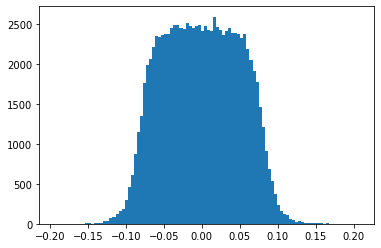
plt.hist(..., bins=100);

TASK 2: \(L_2\) regularization

Create a model like on TASK 1, but include \(L_2\) regularization to every hidden layer (in kernel_regularizer) with a regularization parameter equal to 0.0001.

Use tf.keras.regularizers.L2

def get_L2_model(input_dim, nb_classes):
    from tensorflow.keras.models import Sequential
    from tensorflow.keras.layers import Dense
    from tensorflow.keras import regularizers
    model = ...
    return model

model = get_L2_model(784, 10)
model.summary()

inspect layer regularizers

for layer in model.layers:
    print (layer.name, '-->', layer.kernel_regularizer)

Registra tu solución en linea

student.submit_task(namespace=globals(), task_id='T2');

Run the following cell to train and test the model

from tensorflow.keras import optimizers
model = get_L2_model(784, 10)

# or instantiate an optimizer before passing it to model.compile
sgd = optimizers.SGD(learning_rate=0.01, momentum=0.9, nesterov=True)
model.compile(loss='categorical_crossentropy', optimizer=sgd)
model.fit(X_trainN[:500,:], y_trainOHE[:500,:], epochs=1000, batch_size=16, validation_split=0, verbose=0)

preds = model.predict(X_testN, verbose=0)
preds = np.argmax(preds,axis=1)
Accuracy = np.mean(preds == y_test)
print('Accuracy = %.2f%s'%(Accuracy*100, '%'))

UNGRADED TASK: Create a graph with the histogram of the network weigths in the first hidden layer. It should look like the the following.

Compare it with the histogram obtained in the previous exercise. Is there any effect due to the regularization?

from IPython.display import Image
Image("local/imgs/L21W2.png")

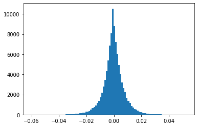
plt.hist(..., bins=100)

TASK 3: \(L_1\)+\(L_2\) regularization

Create a model like on TASK 1, but use \(L_1\)+\(L_2\) regularization to every hidden layer (in kernel_regularizer) with both regularization parameters equal to 0.0001.

Use tf.keras.regularizers.L1L2

def get_L1L2_model(input_dim, nb_classes):
    from tensorflow.keras.models import Sequential
    from tensorflow.keras.layers import Dense
    from tensorflow.keras import regularizers
    model = ...
    return model

model = get_L1L2_model(784, 10)
model.summary()

inspect layer regularizers

for layer in model.layers:
    print (layer.name, '-->', layer.kernel_regularizer)

Registra tu solución en linea

student.submit_task(namespace=globals(), task_id='T3');

Run the following cell to train and test the model

from tensorflow.keras import optimizers
model = get_L1L2_model(784, 10)

# or instantiate an optimizer before passing it to model.compile
sgd = optimizers.SGD(lr=0.01, decay=1e-6, momentum=0.9, nesterov=True)
model.compile(loss='categorical_crossentropy', optimizer=sgd)
model.fit(X_trainN[:500,:], y_trainOHE[:500,:], epochs=1000, batch_size=16, validation_split=0, verbose=0)

preds = model.predict(X_testN, verbose=0)
preds = np.argmax(preds,axis=1)
Accuracy = np.mean(preds == y_test)
print('Accuracy = %.2f%s'%(Accuracy*100, '%'))

UNGRADED TASK: Create a graph with the histogram of the network weigths in the first hidden layer. It should look like the the following.

Compare it with the histograms obtained in the previous exercises. What is the effect of applying \(L_1\) regularization?

from IPython.display import Image
Image("local/imgs/L21W3.png")

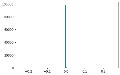
plt.hist(..., bins=100)

Create a graph with the histogram of the network weigths in the first hidden layer. Compare it with the histograms obtained in the previous exercises. What is the effect of applying \(L_1\) regularization?

TASK 4: Customized loss function

Complete the function below to implement the following loss function:

\[\mathcal{L}({\bf{\hat{y}}},{\bf{y}}) = -\frac{1}{N}\sum_{i=1}^N \sum_{j=1}^C {\bf{1}}_{y_i \in C_j} w_{j}\log p_{model}[y_i \in C_j]\]

which corresponds to a weighted version of the categorical cross entropy loss function (take a look to the section 2.2 to remember the notation of the categorical cross-entropy loss function).

Note the following observations:

• the function below returns a function tied to a specific set of weights. This way we can create different loss functions tied to different weights.

• you can assume y_pred to be the output of a softmax layer. This is, that for each y there is a predicted probability for each class \(\in [0,1]\) and summing all up to 1.

• before using the tf.mat.log function, pass y_pred through tf.clip_by_value to ensure any value is between K.epsilon() and 1-K.epsilon(). This is to avoid extreme values close to 0 or close to 1 which might cause numerical issues.

• both y_pred and y_true will be tensors of shape (m,c) with m being the number of data points and c the number of classes.

• your answer must be accurate up to three decimal number.

• use tf.reduce_mean for the first summation, and tf.reduce_sum for the second summation with the corresponding axis argument.

HINT: experiment and understand tf.reduce_mean and tf.reduce_sum before implementing the function

from tensorflow.keras import backend as K
K.epsilon()

z = np.random.randint(100, size=(3,5))
print (z)
print (tf.reduce_mean(z))
print (tf.reduce_sum(z, axis=0))

def weighted_categorical_crossentropy(weights):
    from tensorflow.keras import backend as K
            
    def loss_function(y_true, y_pred):
        # clip y_pred to prevent NaN's and Inf's
        y_pred = ...
        # compute loss
        loss = ...
        return loss
    
    return loss_function

manually test your code with the following cases

y_pred = np.array([[0.14285714, 0.        , 0.68367347, 0.17346939],
                   [0.01020408, 0.60714286, 0.10204082, 0.28061224],
                   [0.1733871 , 0.29435484, 0.24193548, 0.29032258],
                   [0.25403226, 0.24596774, 0.19758065, 0.30241935],
                   [0.52073733, 0.10138249, 0.11981567, 0.25806452],
                   [0.47843137, 0.05882353, 0.24313725, 0.21960784]]).astype(np.float32)

y_true = np.array([[0, 1, 0, 0],
                   [0, 1, 0, 0],
                   [0, 0, 0, 1],
                   [0, 0, 0, 1],
                   [1, 0, 0, 0],
                   [1, 0, 0, 0]]).astype(np.float32)


loss = weighted_categorical_crossentropy([1,1,1,1])
print ("loss", loss(y_true, y_pred).numpy()) # this should return 3.4066
loss = weighted_categorical_crossentropy([2,3,4,5])
print ("loss", loss(y_true, y_pred).numpy()) # this should return 10.7990

test with random data

m,c = np.random.randint(5)+5,np.random.randint(3)+2
y_true = np.eye(c)[np.random.randint(c, size=m)].astype(int)
y_pred = np.abs(y_true + np.round(np.random.random(size=(m,c)),2)*2 - .5)
y_pred[0,np.argmax(y_true[0])]=0 # force some zero to check clipping
y_pred /= np.sum(y_pred,axis=1).reshape(-1,1).astype(np.float32)

w = np.round(np.random.random(size=c)*10+1,2)

print("y_true:\n", y_true)
print("y_pred:\n", y_pred)
print ("w:", w)

loss = weighted_categorical_crossentropy(w)

print ("\nloss: ", loss(y_true, y_pred).numpy())

Registra tu solución en linea

student.submit_task(namespace=globals(), task_id='T4');

UNGRADED TASK

Test your loss function in model. Use the weighted categorical cross entropy function to train the MLP model on the Fashion MNIST dataset with 2 hidden layers of 64 and 32 neurons respectively. Use the two sets of weights below. Evaluate the model with the test dataset and plot the confusion matrix.

Your should get confusion matrices such as the ones below. Left is with weights0, center with weights1 and right with weights2. Observe what classes improve their accuracy based on the weights.

Image("local/imgs/L2.1_W.png")

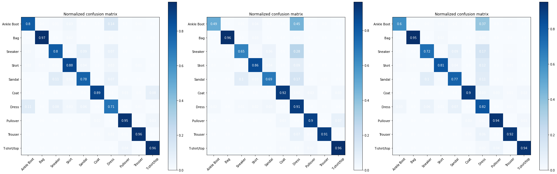
weights0 = np.array([1,1,1,1,1,1,1,1,1,1])
weights1 = np.array([1,1,1,1,1,1,4,1,1,1])
weights2 = np.array([1.5,1,1,1,1,1,4,1,1,1])

def confusion_matrix(y_true, y_pred):
    from sklearn.metrics import confusion_matrix
    objects = ('Ankle Boot', 'Bag', 'Sneaker', 'Shirt', 'Sandal', 'Coat', 'Dress', 'Pullover', 'Trouser', 'T-shirt/top')
    cm = confusion_matrix(y_true, y_pred)
    cm = cm/np.sum(cm,axis=1)
    cmap = plt.cm.Blues
    tick_marks = np.arange(nb_classes)
    fig, ax = plt.subplots(figsize=(10,10))
    im = ax.imshow(cm, interpolation='nearest', cmap=cmap)
    for i in range(cm.shape[0]):
        for j in range(cm.shape[1]):
            text = ax.text(j, i, np.around(cm[i, j],decimals=2),
                           ha="center", va="center", color="w")
    plt.title('Normalized confusion matrix')
    fig.colorbar(im)
    plt.xticks(tick_marks, objects, rotation=45)
    plt.yticks(tick_marks, objects);