
LAB 2.3 - Pairwise classification#
!wget -nc --no-cache -O init.py -q https://raw.githubusercontent.com/rramosp/2021.deeplearning/main/content/init.py
import init; init.init(force_download=False); init.get_weblink()
from local.lib.rlxmoocapi import submit, session
import inspect
session.LoginSequence(endpoint=init.endpoint, course_id=init.course_id, session_id='udea.pre.20252', lab_id="L02.03", varname="student");
LAB SUMMARY#
In this lab we will use define a slightly different machine learning task. Given two MNIST images as input we want a network with a binary output: 1 if both images belong to the same MNIST class, and 0 otherwise.
import pandas as pd
import numpy as np
import matplotlib.pyplot as plt
from sklearn.model_selection import train_test_split
import tensorflow as tf
%matplotlib inline
mnist = pd.read_csv("local/data/mnist1.5k.csv.gz", compression="gzip", header=None).values
X=(mnist[:,1:785]/255.).astype(np.float32)
y=(mnist[:,0]).astype(int)
print("dimension de las imagenes y las clases", X.shape, y.shape)
dimension de las imagenes y las clases (1500, 784) (1500,)
Xtr, Xts, ytr, yts = train_test_split(X,y, test_size=0.3)
Xtr.shape, ytr.shape, Xts.shape, yts.shape
((1050, 784), (1050,), (450, 784), (450,))
FIRST, observe how we build a labelled dataset for this task, so that each training example has:
two images selected randomly from the original dataset
label
0if they belong to the same class, or1otherwise
This way, the resulting data structures
pXtrandpXtscontain the paired images, for train and for testpytrandpytscontain the labels of the corresponding paired images, for train and for testeytrandeytscontain the0/1new labels, one for each pair.
def pairup(X, y, n_pairs_per_class, same_class):

    idxs = None
    labels = np.unique(y)
    for i in labels:
        idxs_p1 = np.argwhere(y==i)[:,0] if same_class else np.argwhere(y!=i)[:,0]
        idxs_p2 = np.argwhere(y==i)[:,0]
        c = np.vstack([
                    np.random.choice(idxs_p1, size=n_pairs_per_class, replace=True),
                    np.random.choice(idxs_p2, size=n_pairs_per_class, replace=True)
            ]).T

        idxs = c if idxs is None else np.vstack((idxs,c))

    X_pairs = [X[idxs[:,0]],X[idxs[:,1]]]
    y_pairs = [y[idxs[:,0]],y[idxs[:,1]]]
    y_labels = y[idxs[:,0]]==y[idxs[:,1]]

    return idxs, X_pairs, y_pairs, y_labels

def build_image_pairs(X,y,n_pairs_per_class):
    idxs0, pX0, py0, ey0 = pairup(X, y, n_pairs_per_class, same_class=False)
    idxs1, pX1, py1, ey1 = pairup(X, y, n_pairs_per_class, same_class=True)

    pX = [np.vstack((i,j)) for i,j in zip(pX0, pX1)]
    py = [np.hstack((i,j)) for i,j in zip(py0, py1)]
    ey = np.hstack((ey0, ey1))
    idxs = np.vstack((idxs0, idxs1))

    return idxs, pX, py, ey.astype(int)
itr, pXtr, pytr, eytr = build_image_pairs(Xtr, ytr, n_pairs_per_class=100)
its, pXts, pyts, eyts = build_image_pairs(Xts, yts, n_pairs_per_class=100)
understand and inspect the structures created and observe how the function above creates a balanced dataset
[i.shape for i in pXtr], [i.shape for i in pytr], itr.shape, eytr.shape
([(2000, 784), (2000, 784)], [(2000,), (2000,)], (2000, 2), (2000,))
[i.shape for i in pXts], [i.shape for i in pyts], its.shape, eyts.shape
([(2000, 784), (2000, 784)], [(2000,), (2000,)], (2000, 2), (2000,))
print ("class distribution %.2f::%.2f"%(np.mean(eytr), 1-np.mean(eytr)))
class distribution 0.50::0.50
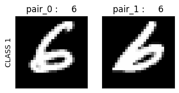
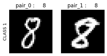
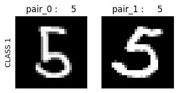
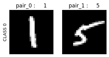
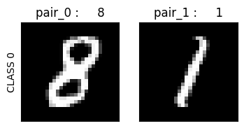
for _ in range(5):
    i = np.random.randint(len(pXtr[0]))
    plt.figure(figsize=(4,2))
    plt.subplot(121)
    plt.imshow(pXtr[0][i].reshape(28,28), cmap=plt.cm.Greys_r);
    plt.ylabel("CLASS %d"%(eytr[i]));
    plt.title("pair_0 :     %d"%(pytr[0][i])); plt.xticks([],[]); plt.yticks([],[])
    plt.subplot(122)
    plt.imshow(pXtr[1][i].reshape(28,28), plt.cm.Greys_r);
    plt.title("pair_1 :     %d"%pytr[1][i]); plt.xticks([],[]); plt.yticks([],[])
TASK 1: Multi-input model#
Create a model with the architecture depicted in the following figure.
from IPython.display import Image
Image(filename='local/imgs/twoinputs.png', width=600)
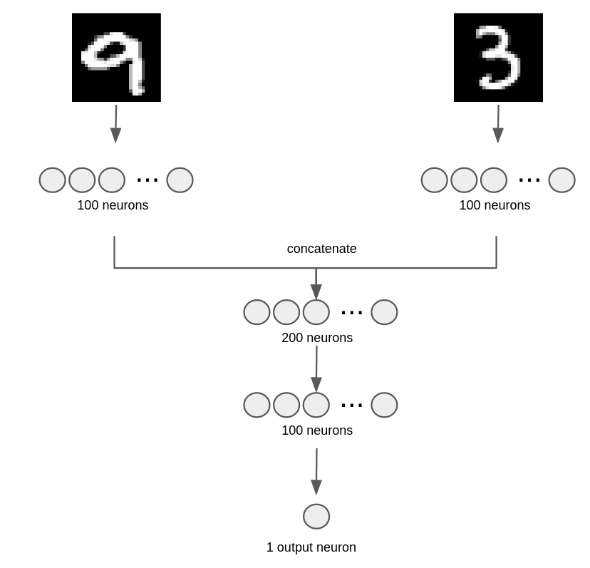
Observe that
it will have TWO input layers with
input_dim=784neurons each.there is ony ONE output neuron.
the model summary should be as follows and MUST NAME THE LAYERS ACCORDINGLY. For concatenation just use the class
Concatprovided:
┏━━━━━━━━━━━━━━━━━━━━━┳━━━━━━━━━━━━━━━━━━━┳━━━━━━━━━━━━┳━━━━━━━━━━━━━━━━━━━┓
┃ Layer (type)        ┃ Output Shape      ┃    Param # ┃ Connected to      ┃
┡━━━━━━━━━━━━━━━━━━━━━╇━━━━━━━━━━━━━━━━━━━╇━━━━━━━━━━━━╇━━━━━━━━━━━━━━━━━━━┩
│ input_img0          │ (None, 784)       │          0 │ -                 │
│ (InputLayer)        │                   │            │                   │
├─────────────────────┼───────────────────┼────────────┼───────────────────┤
│ input_img1          │ (None, 784)       │          0 │ -                 │
│ (InputLayer)        │                   │            │                   │
├─────────────────────┼───────────────────┼────────────┼───────────────────┤
│ layer1_img0 (Dense) │ (None, 100)       │     78,500 │ input_img0[0][0]  │
├─────────────────────┼───────────────────┼────────────┼───────────────────┤
│ layer1_img1 (Dense) │ (None, 100)       │     78,500 │ input_img1[0][0]  │
├─────────────────────┼───────────────────┼────────────┼───────────────────┤
│ concat (Concat)     │ (None, 200)       │          0 │ layer1_img0[0][0… │
│                     │                   │            │ layer1_img1[0][0] │
├─────────────────────┼───────────────────┼────────────┼───────────────────┤
│ layer2_common       │ (None, 100)       │     20,100 │ concat[0][0]      │
│ (Dense)             │                   │            │                   │
├─────────────────────┼───────────────────┼────────────┼───────────────────┤
│ output (Dense)      │ (None, 1)         │        101 │ layer2_common[0]… │
└─────────────────────┴───────────────────┴────────────┴───────────────────┘

 Total params: 177,201 (692.19 KB)
 Trainable params: 177,201 (692.19 KB)
 Non-trainable params: 0 (0.00 B)
def get_model(input_dim):

    class Concat(tf.keras.Layer):
        def call(self, layers):
            return tf.concat(layers,axis=1)

    inputs1  = tf.keras.layers.Input(shape=(input_dim,), name="input_img0")
    inputs2  = tf.keras.layers.Input(shape=(input_dim,), name="input_img1")

    ...

    outputs = ...

    model = tf.keras.Model(inputs=[inputs1, inputs2], outputs=outputs)
    model.compile(optimizer='adam', loss='mse')
    return model
model = get_model(X.shape[1])
model.summary()
Registra tu solución en linea
student.submit_task(namespace=globals(), task_id='T1');
test your model
now we can test your model
model = get_model(X.shape[1])
model.fit(pXtr, eytr, batch_size=16, epochs=20)
preds_ts = (model.predict(pXts)[:,0]>.5).astype(int)
preds_tr = (model.predict(pXtr)[:,0]>.5).astype(int)
print ("accuracy in train data %.2f"%(np.mean(preds_tr==eytr)))
print ("accuracy in test data  %.2f"%(np.mean(preds_ts==eyts)))
inspect TEST predictions. Do you see any class getting more confused with others?
for _ in range(20):
    i = np.random.randint(len(pXts[0]))
    plt.figure(figsize=(4,2))
    plt.subplot(121)
    plt.imshow(pXts[0][i].reshape(28,28), cmap=plt.cm.Greys_r)
    plt.ylabel("PREDICTION %d\nTARGET %d"%(preds_ts[i], eyts[i]))
    plt.subplot(122)
    plt.imshow(pXts[1][i].reshape(28,28), cmap=plt.cm.Greys_r)
TASK 2: Measure per-class accuracy#
For each class we want to measure what is the prediction accuracy for the binary task when it participates in a pair. Observe how we gather the labels of each pair together with the binary prediction and the true value.
ts = pd.DataFrame(np.vstack((pyts[0],pyts[1], eyts, preds_ts)).T, columns=["pair_0", "pair_1", "true", "pred"])
ts.head()
| pair_0 | pair_1 | true | pred | |
|---|---|---|---|---|
| 0 | 6 | 0 | 0 | 1 |
| 1 | 7 | 0 | 0 | 0 |
| 2 | 5 | 0 | 0 | 1 |
| 3 | 4 | 0 | 0 | 0 |
| 4 | 7 | 0 | 0 | 0 |
of course, the true value coincides with pair_0 being equal or different from pair_1.
np.mean((ts.pair_0==ts.pair_1)==ts.true)
np.float64(1.0)
To compute, per-class accuracy in this task, for instance for class 2:
select the rows where
pair_0orpair_1is 2measure the percentage of time in the selected rows where
true==pred
for instance, for the following DataFrame
        pair_0  pair_1  true  pred
    0        0       0     1     1
    1        0       0     1     1
    2        0       0     1     1
    3        2       2     1     1
    4        1       1     1     1
    5        0       2     0     0
    6        2       2     1     0
    7        2       2     1     1
    8        2       2     1     1
    9        1       1     1     1
    10       1       1     1     1
    11       1       1     1     1
    12       2       2     1     1
    13       0       2     0     1
    14       2       2     1     1
    15       0       0     1     1
    16       2       2     1     1
    17       1       1     1     0
    18       1       1     1     1
    19       1       1     1     1
you must return this accuracies:
{0: 0.8333333333333334, 1: 0.8571428571428571, 2: 0.7777777777777778}
the accuracies must be returned as a dictionary such as above. They keys are the original class labels, and the values the accuracy just described.
The accuracies must be correct up to 3 decimal values.
def perclass_bin_accuracy(ts):

    r = {}
    for i in np.unique(ts.pair_0.tolist() + ts.pair_1.tolist()):
        ...
        r[i] = ... # your code here

    return r
test your code with the example above
t = pd.DataFrame(
        np.array([[0, 0, 1, 1],[0, 0, 1, 1],[0, 0, 1, 1],[2, 2, 1, 1],[1, 1, 1, 1],
                  [0, 2, 0, 0],[2, 2, 1, 0],[2, 2, 1, 1],[2, 2, 1, 1],[1, 1, 1, 1],[1, 1, 1, 1],[1, 1, 1, 1],
                  [2, 2, 1, 1],[0, 2, 0, 1],[2, 2, 1, 1],[0, 0, 1, 1],[2, 2, 1, 1],[1, 1, 1, 0],[1, 1, 1, 1],
                  [1, 1, 1, 1]]),
    columns=["pair_0", "pair_1", "true", "pred"])
perclass_bin_accuracy(t)
test your code with other random examples
n, n_classes = 20, 3
p0 = np.random.randint(n_classes, size=n)
p1 = np.random.randint(n_classes, size=n)
dtrue = (p0==p1).astype(int)
preds = np.random.randint(2, size=n)
td = pd.DataFrame([p0,p1,dtrue,preds], index=["pair_0", "pair_1", "true", "pred"]).T

td
perclass_bin_accuracy(td)
Registra tu solución en linea
student.submit_task(namespace=globals(), task_id='T2');