
5.1 Recurrent Neural Networks#
!wget -nc --no-cache -O init.py -q https://raw.githubusercontent.com/rramosp/2021.deeplearning/main/content/init.py
import init; init.init(force_download=False);
from IPython.core.display import display, HTML
display(HTML("<style>.container {width:100% !important;}</style>"))
%matplotlib inline
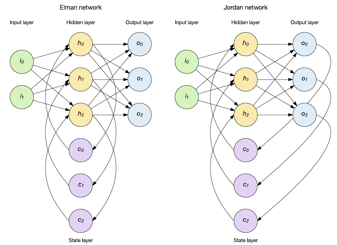
Recurrent Neural Networks (RNN) are a family of neural networks designed to process sequential data. This type of networks are specially suitable for problems where every sample is a sequence of objects (values) with statistical dependence among them.
from IPython.display import Image
Image(filename='local/imgs/RNN2.png', width=700)
RNNs can be designed to solve different learning paradigms, in other words, they are able to adapt to different data configurations.
Image(filename='local/imgs/RNN-Topol.jpeg', width=1200)
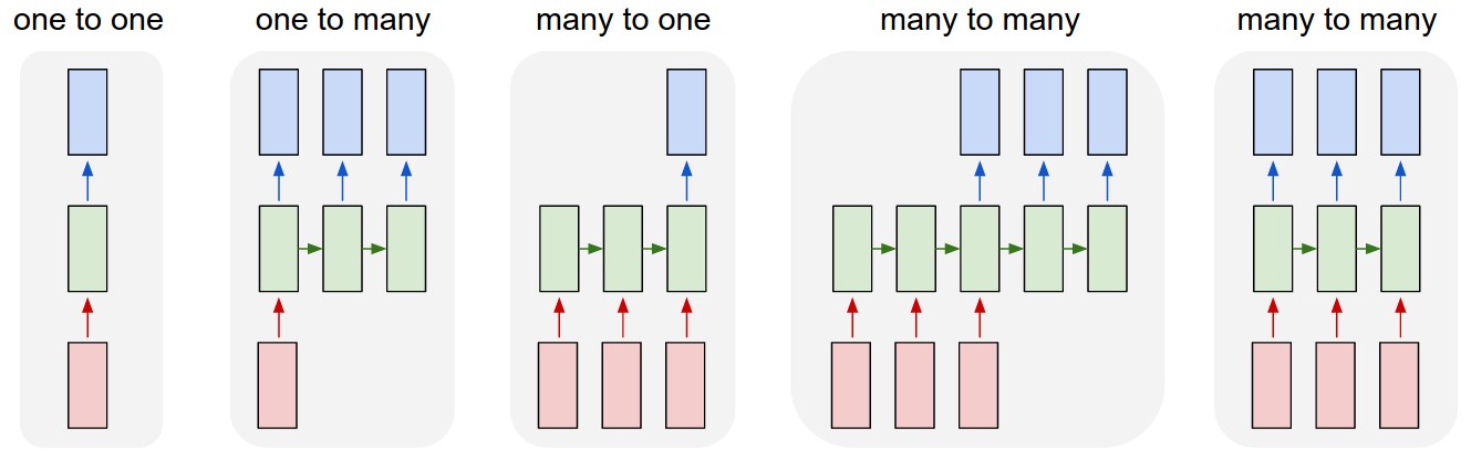
Image taken from Andrej Karpathy
Examples:
Conventional MLP
Caption generation
Sentiment analysis
Language translation
Named Entity Recognition or Part Of Speech Tagging
Lets do some examples of Time series using conventional MLPs#
First we need some data:
import warnings
warnings.filterwarnings('ignore')
from tensorflow.keras.models import Sequential
from tensorflow.keras.layers import Dense, Dropout, SimpleRNN, RepeatVector, TimeDistributed, LSTM
from tensorflow import keras
from local.lib import DataPreparationRNN
import pandas as pd
import numpy as np
import matplotlib.pyplot as plt
from local.lib.DataPreparationRNN import split_sequence
from sklearn.preprocessing import MinMaxScaler

datasetO = pd.read_csv('local/data/international-airline-passengers.csv', usecols=[1], engine='python', skipfooter=3)
dataset = datasetO.values
dataset = dataset.astype('float32')
len(dataset)
144
For simplicity we are going to split the data manualy into training and validation sets using the classical approach
look_back=2
# split into train and test sets
train_size = int(len(dataset) * 0.67)
test_size = len(dataset) - train_size
train, test = dataset[0:train_size], dataset[train_size:len(dataset)]

# normalize the dataset
scaler = MinMaxScaler(feature_range=(0, 1))
trainN = scaler.fit_transform(train)
testN = scaler.transform(test)

#tensor formating

X_train, y_train = split_sequence(trainN, look_back)
X_test, y_test = split_sequence(testN, look_back)
print('Train',X_train[:10])
print('Test',y_train[:10])
Train [[[0.02588999]
  [0.04530746]]

 [[0.04530746]
  [0.09061491]]

 [[0.09061491]
  [0.08090615]]

 [[0.08090615]
  [0.05501619]]

 [[0.05501619]
  [0.10032365]]

 [[0.10032365]
  [0.14239484]]

 [[0.14239484]
  [0.14239484]]

 [[0.14239484]
  [0.10355988]]

 [[0.10355988]
  [0.04854369]]

 [[0.04854369]
  [0.        ]]]
Test [[0.09061491]
 [0.08090615]
 [0.05501619]
 [0.10032365]
 [0.14239484]
 [0.14239484]
 [0.10355988]
 [0.04854369]
 [0.        ]
 [0.04530746]]
X_train.shape, y_train.shape
((94, 2, 1), (94, 1))
X_test.shape
(46, 2, 1)
Let’s create the MLP.
#keras.backend.clear_session()
model1 = Sequential()
model1.add(Dense(5,activation = 'relu',input_dim=look_back))
model1.add(Dense(1))
model1.summary()
Model: "sequential_1"
_________________________________________________________________
Layer (type)                 Output Shape              Param #
=================================================================
dense_2 (Dense)              (None, 5)                 15
_________________________________________________________________
dense_3 (Dense)              (None, 1)                 6
=================================================================
Total params: 21
Trainable params: 21
Non-trainable params: 0
_________________________________________________________________
model1.compile(optimizer='adam',loss='mse')
model1.fit(X_train.reshape(X_train.shape[0],look_back),y_train.flatten(),epochs=200, verbose=0)
trainPredict, testPredict = DataPreparationRNN.EstimaRMSE(model1,X_train,X_test,y_train,y_test,scaler,look_back)
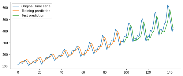
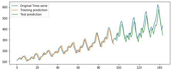
DataPreparationRNN.PintaResultado(dataset,trainPredict,testPredict,look_back)
Train Score: 28.23 RMSE
Test Score: 61.99 RMSE
Train Score: 10.23 MAPE
Test Score: 12.50 MAPE
1
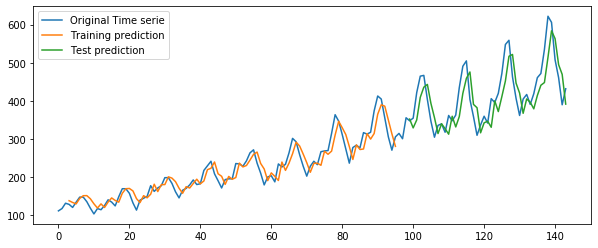
Using three steps backward to predict one step ahead:#
look_back = 3;
X_train, y_train = split_sequence(trainN, look_back)
X_test, y_test = split_sequence(testN, look_back)

#Model
model3 = Sequential()
model3.add(Dense(5,activation = 'relu',input_dim=look_back))
model3.add(Dense(1))
model3.compile(optimizer='adam',loss='mse')
model3.fit(X_train.reshape(X_train.shape[0],look_back),y_train.flatten(),epochs=200, verbose=0)

#Validation
trainPredict, testPredict = DataPreparationRNN.EstimaRMSE(model3,X_train,X_test,y_train,y_test,scaler,look_back)
DataPreparationRNN.PintaResultado(dataset,trainPredict,testPredict,look_back)
Train Score: 23.14 RMSE
Test Score: 50.44 RMSE
Train Score: 8.56 MAPE
Test Score: 10.10 MAPE
1
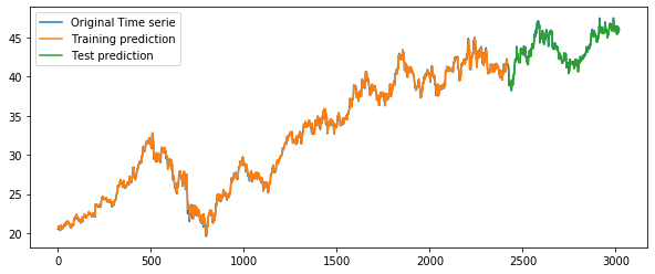
look_back=3
dataset1 = pd.read_csv('local/data/KO_2006-01-01_to_2018-01-01.csv', usecols=['High'])
dataset1[np.isnan(dataset1)] = dataset1['High'].max()
dataset = dataset1.values
dataset = dataset.astype('float32')
# split into train and test sets
test_size = 600
train_size = int(len(dataset) - test_size)
train, test = dataset[0:train_size], dataset[train_size:len(dataset)]
# normalize the dataset
scaler = MinMaxScaler(feature_range=(0, 1))
trainN = scaler.fit_transform(train)
testN = scaler.transform(test)
X_train, y_train = split_sequence(trainN, look_back)
X_test, y_test = split_sequence(testN, look_back)
#------------------------------------------------------------------
keras.backend.clear_session()
model3b = Sequential()
model3b.add(Dense(30,activation = 'relu',input_dim=look_back))
model3b.add(Dense(1))
model3b.compile(optimizer='adam',loss='mse')
model3b.fit(X_train.reshape(X_train.shape[0],look_back),y_train.flatten(),epochs=50, verbose=0)
trainPredict, testPredict = DataPreparationRNN.EstimaRMSE(model3b,X_train,X_test,y_train,y_test,scaler,look_back)
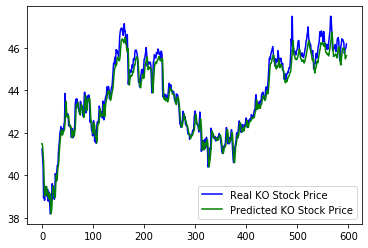
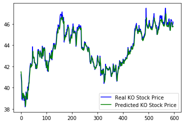
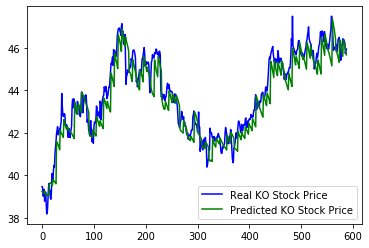
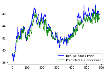
DataPreparationRNN.PintaResultado(dataset,trainPredict,testPredict,look_back)
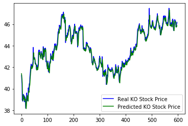
Train Score: 0.42 RMSE
Test Score: 0.48 RMSE
Train Score: 0.99 MAPE
Test Score: 0.85 MAPE
1

plt.plot(scaler.inverse_transform(y_test),'b',label='Real KO Stock Price')
plt.plot(testPredict,'g',label='Predicted KO Stock Price')
plt.legend()
plt.show()
There are also problems with basic MLP when we have multiple time series to forecast one of them (Multiple Input series), or multiple time series to predict all of them (Multiple parallel series)
Let’s define formaly the Recurrent Neural Networks#
An alternative view of the network
from IPython.display import Image
Image(filename='local/imgs/RNN3.png', width=1200)
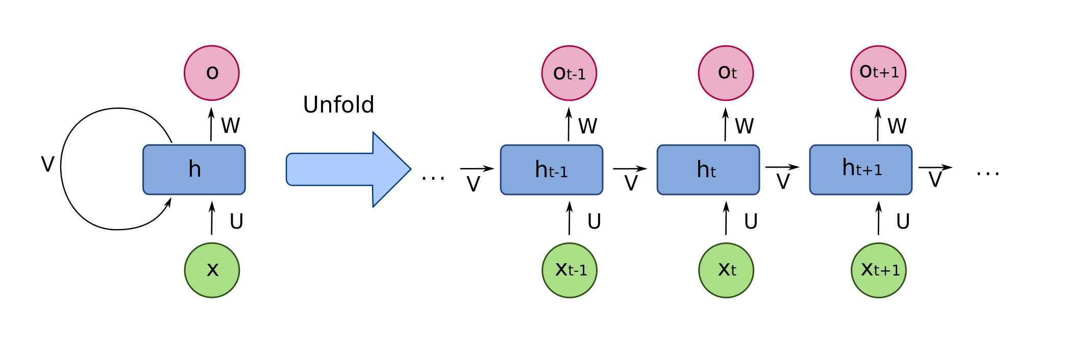
According to the notation in the in the former Figure, the mathematical formulation of an Elman RNN with one hidden layer and one output layer is given by:
where \(\bf{V}\) is the weights matrix of the feedback loop. \(\bf{U}\) is the weights matrix of the inputs and \(\bf{W}\) is the weights matrix that contects the state of the network with the output layer. \(\bf{b}\) and \(\bf{c}\) are the bias vectors for the hidden and output layers respectively. The ouput of the network \({\bf{y}}^{(t)}\) corresponds to the application of the activation function to the values \({\bf{o}}^{(t)}\).
Backpropagation through time (BPTT)#
The first step for training a RNN is to define the loss function. Let’s consider a sequence of length \(\tau\), the loss for that single sequence can be expressed as:
If for instance the loss function for output \(i\) is \(L^{(t)} = -\log \hat{y}_i^{(t)}\), then
where \(\odot\) is the Hadamard product. When \(t=\tau\), \({\bf{h}}^{(\tau)}\) only has \({\bf{o}}^{(\tau)}\) as descendent, so its gradient is simple:
From this two results we can iterate backward in time to back-propagate gradients through time. From \(t=\tau-1\) down to \(\tau = 1\), \({\bf{h}}^{(t)}\) has two descendents: \({\bf{h}}^{(t+1)}\) and \({\bf{o}}^{(t)}\), therefore its gradient is given by:
Based on the former results, the rest of the gradients can be calculated as:
Now using a RNN layer instead of a Dense layer:#
Input data must have the following structure: [n_samples,n_times,n_features]
Input: [n_samples,1,1]
look_back = 1;
dataset = datasetO.values
dataset = dataset.astype('float32')

# split into train and test sets
train_size = int(len(dataset) * 0.67)
test_size = len(dataset) - train_size
train, test = dataset[0:train_size], dataset[train_size:len(dataset)]

# normalize the dataset
scaler = MinMaxScaler(feature_range=(0, 1))
trainN = scaler.fit_transform(train)
testN = scaler.transform(test)
X_train, y_train = DataPreparationRNN.create_dataset(trainN, look_back)
X_test, y_test = DataPreparationRNN.create_dataset(testN, look_back)
X_train.shape
(95, 1)
model4 = Sequential()
model4.add(SimpleRNN(5,activation = 'relu',input_shape=(1,look_back)))
model4.add(Dense(1))

model4.compile(optimizer='adam',loss='mse')
model4.fit(X_train.reshape(X_train.shape[0],1,look_back),y_train.flatten(),epochs=500, verbose=0)
trainPredict, testPredict = DataPreparationRNN.EstimaRMSE_RNN(model4,X_train,X_test,y_train,y_test,scaler,look_back,1)
DataPreparationRNN.PintaResultado(dataset,trainPredict,testPredict,look_back)
Train Score: 22.88 RMSE
Test Score: 48.72 RMSE
Train Score: 8.51 MAPE
Test Score: 9.78 MAPE
1
model4.summary()
Model: "sequential_4"
_________________________________________________________________
Layer (type)                 Output Shape              Param #
=================================================================
simple_rnn_2 (SimpleRNN)     (None, 5)                 35
_________________________________________________________________
dense_6 (Dense)              (None, 1)                 6
=================================================================
Total params: 41
Trainable params: 41
Non-trainable params: 0
_________________________________________________________________
Using multiple times as features#
Input: [n_samples,1,2]
look_back = 2;
X_train, y_train = DataPreparationRNN.create_dataset(trainN, look_back)
X_test, y_test = DataPreparationRNN.create_dataset(testN, look_back)
#-----------------------------------------------------------------
model4b = Sequential()
model4b.add(SimpleRNN(5,activation = 'relu',input_shape=(1,look_back)))
model4b.add(Dense(1))
#-------------------------------------------------------------------

model4b.compile(optimizer='adam',loss='mse')
model4b.fit(X_train.reshape(X_train.shape[0],1,look_back),y_train.flatten(),epochs=500, verbose=0)
trainPredict, testPredict = DataPreparationRNN.EstimaRMSE_RNN(model4b,X_train,X_test,y_train,y_test,scaler,look_back,1)
DataPreparationRNN.PintaResultado(dataset,trainPredict,testPredict,look_back)
Train Score: 26.23 RMSE
Test Score: 53.59 RMSE
Train Score: 9.60 MAPE
Test Score: 10.65 MAPE
1
model4b.summary()
Model: "sequential_2"
_________________________________________________________________
Layer (type)                 Output Shape              Param #
=================================================================
simple_rnn_1 (SimpleRNN)     (None, 5)                 40
_________________________________________________________________
dense_3 (Dense)              (None, 1)                 6
=================================================================
Total params: 46
Trainable params: 46
Non-trainable params: 0
_________________________________________________________________
Using multiple times instead of multiple features:
Using multiple times as multiple times!#
Input: [n_samples,2,1]
n_steps = 2;
X_train, y_train = DataPreparationRNN.create_dataset(trainN, n_steps)
X_test, y_test = DataPreparationRNN.create_dataset(testN, n_steps)
#---------------------------------------------------------------------
model6 = Sequential()
model6.add(SimpleRNN(5,activation = 'relu',input_shape=(n_steps,1)))
model6.add(Dense(1))
#---------------------------------------------------------------------
model6.compile(optimizer='adam',loss='mse')
model6.fit(X_train.reshape(X_train.shape[0],n_steps,1),y_train.flatten(),epochs=500, verbose=0)
#-----------------------------------------------------------------------------------------------------
trainPredict, testPredict = DataPreparationRNN.EstimaRMSE_RNN(model6,X_train,X_test,y_train,y_test,scaler,1,n_steps)
DataPreparationRNN.PintaResultado(dataset,trainPredict,testPredict,n_steps)
Train Score: 21.17 RMSE
Test Score: 51.46 RMSE
Train Score: 8.26 MAPE
Test Score: 9.29 MAPE
1
model6.summary()
Model: "sequential_8"
_________________________________________________________________
Layer (type)                 Output Shape              Param #
=================================================================
simple_rnn_7 (SimpleRNN)     (None, 5)                 35
_________________________________________________________________
dense_9 (Dense)              (None, 1)                 6
=================================================================
Total params: 41
Trainable params: 41
Non-trainable params: 0
_________________________________________________________________
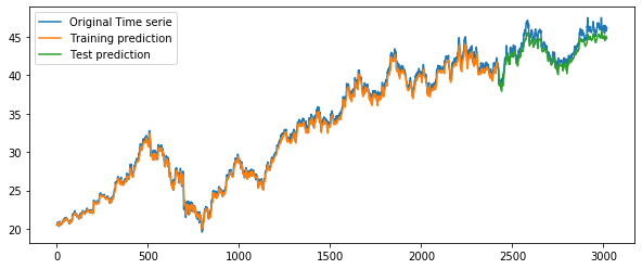
n_steps = 3;
dataset = dataset1.values
dataset = dataset.astype('float32')
# split into train and test sets
test_size = 600
train_size = int(len(dataset) - test_size)
train, test = dataset[0:train_size], dataset[train_size:len(dataset)]
# normalize the dataset
scaler = MinMaxScaler(feature_range=(0, 1))
trainN = scaler.fit_transform(train)
testN = scaler.transform(test)
X_train, y_train = DataPreparationRNN.create_dataset(trainN, n_steps)
X_test, y_test = DataPreparationRNN.create_dataset(testN, n_steps)
#---------------------------------------------------------------------
model6 = Sequential()
model6.add(SimpleRNN(30,activation = 'relu',input_shape=(n_steps,1)))
model6.add(Dense(1))
model6.compile(optimizer='adam',loss='mse')
#-----------------------------------------------------------------------
model6.fit(X_train.reshape(X_train.shape[0],n_steps,1),y_train.flatten(),verbose=0,epochs=50,batch_size=32)
trainPredict, testPredict = DataPreparationRNN.EstimaRMSE_RNN(model6,X_train,X_test,y_train,y_test,scaler,1,n_steps)
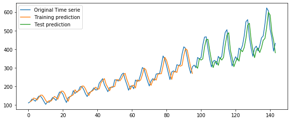
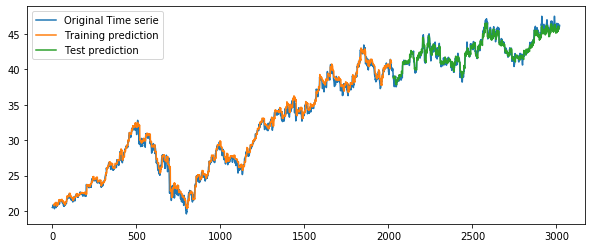
DataPreparationRNN.PintaResultado(dataset,trainPredict,testPredict,n_steps)
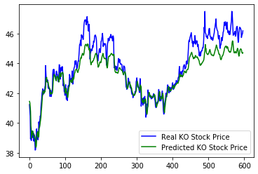
Train Score: 0.31 RMSE
Test Score: 0.35 RMSE
Train Score: 0.70 MAPE
Test Score: 0.59 MAPE
1

plt.plot(scaler.inverse_transform(y_test[:, np.newaxis]),'b',label='Real KO Stock Price')
plt.plot(testPredict.flatten(),'g',label='Predicted KO Stock Price')
plt.legend()
plt.show()
Lets make more complex architectures#
Two recurrent layers:#
Image(filename='local/imgs/ReturnSeq.jpg', width=800)
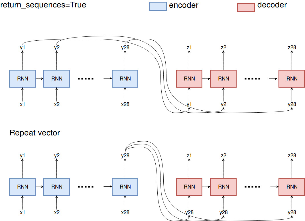
Input: [n_samples,1,1]
Option1: Propagate the first layer and provide every output of the first layer to the following layer:
look_back = 2;
dataset = datasetO.values
dataset = dataset.astype('float32')
# split into train and test sets
train_size = int(len(dataset) * 0.67)
test_size = len(dataset) - train_size
train, test = dataset[0:train_size], dataset[train_size:len(dataset)]
# normalize the dataset
scaler = MinMaxScaler(feature_range=(0, 1))
trainN = scaler.fit_transform(train)
testN = scaler.transform(test)
X_train, y_train = DataPreparationRNN.create_dataset(trainN, look_back)
X_test, y_test = DataPreparationRNN.create_dataset(testN, look_back)
X_train.shape
(94, 2)
temp = X_train.reshape(X_train.shape[0],look_back,1)
temp.shape
(94, 2, 1)
model5b = Sequential()
model5b.add(SimpleRNN(5,activation = 'relu',return_sequences=True,input_shape=(look_back,1)))
model5b.add(SimpleRNN(5,activation = 'relu'))
model5b.add(Dense(1))
#-----------------------------------------------------------------------------------------------
model5b.compile(optimizer='adam',loss='mse')
model5b.fit(X_train.reshape(X_train.shape[0],look_back,1),y_train.flatten(),epochs=500, verbose=0)
trainPredict, testPredict = DataPreparationRNN.EstimaRMSE_RNN(model5b,X_train,X_test,y_train,y_test,scaler,1,look_back)
DataPreparationRNN.PintaResultado(dataset,trainPredict,testPredict,look_back)
Train Score: 26.23 RMSE
Test Score: 67.27 RMSE
Train Score: 9.69 MAPE
Test Score: 12.05 MAPE
1
model5b.summary()
Model: "sequential_7"
_________________________________________________________________
Layer (type)                 Output Shape              Param #
=================================================================
simple_rnn_14 (SimpleRNN)    (None, 2, 5)              35
_________________________________________________________________
simple_rnn_15 (SimpleRNN)    (None, 5)                 55
_________________________________________________________________
dense_7 (Dense)              (None, 1)                 6
=================================================================
Total params: 96
Trainable params: 96
Non-trainable params: 0
_________________________________________________________________
look_back = 3;
dataset = dataset1.values
dataset = dataset.astype('float32')
# split into train and test sets
test_size = 600
train_size = int(len(dataset) - test_size)
train, test = dataset[0:train_size], dataset[train_size:len(dataset)]
# normalize the dataset
scaler = MinMaxScaler(feature_range=(0, 1))
trainN = scaler.fit_transform(train)
testN = scaler.transform(test)
X_train, y_train = DataPreparationRNN.create_dataset(trainN, look_back)
X_test, y_test = DataPreparationRNN.create_dataset(testN, look_back)
#-----------------------------------------------------------------------
model5b = Sequential()
model5b.add(SimpleRNN(20,activation = 'relu',return_sequences=True,input_shape=(look_back,1)))
model5b.add(SimpleRNN(20,activation = 'relu'))
model5b.add(Dense(1))
#-----------------------------------------------------------------------------------------
model5b.compile(optimizer='adam',loss='mse')
model5b.fit(X_train.reshape(X_train.shape[0],look_back,1),y_train.flatten(),epochs=50, validation_split=0.10, verbose=0)
trainPredict, testPredict = DataPreparationRNN.EstimaRMSE_RNN(model5b,X_train,X_test,y_train,y_test,scaler,1,look_back)
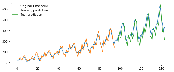
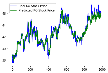
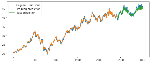
DataPreparationRNN.PintaResultado(dataset,trainPredict,testPredict,look_back)
Train Score: 0.30 RMSE
Test Score: 0.32 RMSE
Train Score: 0.68 MAPE
Test Score: 0.54 MAPE
1
plt.plot(scaler.inverse_transform(y_test[:, np.newaxis]),'b',label='Real KO Stock Price')
plt.plot(testPredict.flatten(),'g',label='Predicted KO Stock Price')
plt.legend()
plt.show()
Option2: Propagate the first layer and provide only the output of the last time step to the following layer:
look_back = 2;
dataset = datasetO.values
dataset = dataset.astype('float32')
# split into train and test sets
train_size = int(len(dataset) * 0.67)
test_size = len(dataset) - train_size
train, test = dataset[0:train_size], dataset[train_size:len(dataset)]
# normalize the dataset
scaler = MinMaxScaler(feature_range=(0, 1))
trainN = scaler.fit_transform(train)
testN = scaler.transform(test)
X_train, y_train = DataPreparationRNN.create_dataset(trainN, look_back)
X_test, y_test = DataPreparationRNN.create_dataset(testN, look_back)
model5 = Sequential()
model5.add(SimpleRNN(5,activation = 'relu',input_shape=(1,look_back)))
model5.add(RepeatVector(look_back))
model5.add(SimpleRNN(5,activation = 'relu'))
model5.add(Dense(1))
#-------------------------------------------------------------------------
model5.compile(optimizer='adam',loss='mse')
model5.fit(X_train.reshape(X_train.shape[0],1,look_back),y_train.flatten(),epochs=500, verbose=0)
trainPredict, testPredict = DataPreparationRNN.EstimaRMSE_RNN(model5,X_train,X_test,y_train,y_test,scaler,look_back,1)
DataPreparationRNN.PintaResultado(dataset,trainPredict,testPredict,look_back)
Train Score: 23.85 RMSE
Test Score: 51.97 RMSE
Train Score: 8.78 MAPE
Test Score: 10.55 MAPE
1

model5.summary()
Model: "sequential_6"
_________________________________________________________________
Layer (type)                 Output Shape              Param #
=================================================================
simple_rnn_5 (SimpleRNN)     (None, 5)                 40
_________________________________________________________________
repeat_vector (RepeatVector) (None, 2, 5)              0
_________________________________________________________________
simple_rnn_6 (SimpleRNN)     (None, 5)                 55
_________________________________________________________________
dense_6 (Dense)              (None, 1)                 6
=================================================================
Total params: 101
Trainable params: 101
Non-trainable params: 0
_________________________________________________________________
look_back = 3;
dataset = dataset1.values
dataset = dataset.astype('float32')
# split into train and test sets
test_size = 600
train_size = int(len(dataset) - test_size)
train, test = dataset[0:train_size], dataset[train_size:len(dataset)]
# normalize the dataset
scaler = MinMaxScaler(feature_range=(0, 1))
trainN = scaler.fit_transform(train)
testN = scaler.transform(test)
X_train, y_train = DataPreparationRNN.create_dataset(trainN, look_back)
X_test, y_test = DataPreparationRNN.create_dataset(testN, look_back)
#---------------------------------------------------------------------
model5 = Sequential()
model5.add(SimpleRNN(20,activation = 'relu',input_shape=(look_back,1)))
model5.add(RepeatVector(look_back))
model5.add(SimpleRNN(20,activation = 'relu',kernel_regularizer=keras.regularizers.l2(0.01)))
model5.add(Dense(1))
#----------------------------------------------------------------------
model5.compile(optimizer='adam',loss='mse')
model5.fit(X_train.reshape(X_train.shape[0],look_back,1),y_train.flatten(),epochs=50, validation_split=0.10,verbose=0)
trainPredict, testPredict = DataPreparationRNN.EstimaRMSE_RNN(model5,X_train,X_test,y_train,y_test,scaler,1,look_back)
DataPreparationRNN.PintaResultado(dataset,trainPredict,testPredict,look_back)
Train Score: 0.50 RMSE
Test Score: 0.92 RMSE
Train Score: 1.21 MAPE
Test Score: 1.83 MAPE
1
plt.plot(scaler.inverse_transform(y_test[:, np.newaxis]),'b',label='Real KO Stock Price')
plt.plot(testPredict.flatten(),'g',label='Predicted KO Stock Price')
plt.legend()
plt.show()
Predicting several times ahead#
Walk forward using a RNN#
look_back = 10
time_ahead = 7
dataset = dataset1.values
dataset = dataset.astype('float32')

# split into train and test sets
test_size = 600
train_size = int(len(dataset) - test_size)
train, test = dataset[0:train_size], dataset[train_size:len(dataset)]

# normalize the dataset
scaler = MinMaxScaler(feature_range=(0, 1))
trainN = scaler.fit_transform(train)
testN = scaler.transform(test)

X_train, y_train = split_sequence(trainN, look_back)
X_test, y_test = DataPreparationRNN.create_datasetMultipleTimesBackAhead(testN, n_steps_out=time_ahead, n_steps_in = look_back, overlap = time_ahead)

model6c = Sequential()
model6c.add(SimpleRNN(20,activation = 'relu',input_shape=(look_back,1)))
model6c.add(Dense(1))


model6c.compile(optimizer='adam',loss='mse')
model6c.fit(X_train.reshape(X_train.shape[0],look_back,1),y_train.flatten(),epochs=500, verbose=0)
trainPredict, testPredict = DataPreparationRNN.EstimaRMSE_RNN_MultiStep(model6c,X_train,X_test,y_train,y_test,scaler,look_back,time_ahead,0)
DataPreparationRNN.PintaResultado(dataset,trainPredict,testPredict,look_back)
Train Score: 0.29 RMSE
Test Score: 0.71 RMSE
Train Score: 0.65 MAPE
Test Score: 1.24 MAPE
3

plt.plot(scaler.inverse_transform(y_test.flatten()[:, np.newaxis]),'b',label='Real KO Stock Price')
plt.plot(testPredict.flatten(),'g',label='Predicted KO Stock Price')
plt.legend()
plt.show()
A RNN network with multiple outputs#
look_back = 10;
time_ahead = 7
dataset = dataset1.values
dataset = dataset.astype('float32')

# split into train and test sets
train_size = int(len(dataset) * 0.67)
test_size = len(dataset) - train_size
train, test = dataset[0:train_size], dataset[train_size:len(dataset)]

# normalize the dataset
scaler = MinMaxScaler(feature_range=(0, 1))
trainN = scaler.fit_transform(train)
testN = scaler.transform(test)

X_train, y_train = DataPreparationRNN.create_datasetMultipleTimesBackAhead(trainN, n_steps_out=time_ahead, n_steps_in = look_back, overlap = time_ahead)
X_train2, y_train2 = DataPreparationRNN.create_datasetMultipleTimesBackAhead(trainN, n_steps_out=time_ahead, n_steps_in = look_back, overlap = 1)
X_test, y_test = DataPreparationRNN.create_datasetMultipleTimesBackAhead(testN, n_steps_out=time_ahead, n_steps_in = look_back, overlap = time_ahead)
print('Train',X_train[:10])
print('Test',y_train[:10])
Train [[0.03776747 0.03944606 0.04028529 0.04951739 0.05203521 0.05287451
  0.05455303 0.05119592 0.04951739 0.0436424 ]
 [0.05119592 0.04951739 0.0436424  0.03776747 0.04070497 0.03524965
  0.03063363 0.04196388 0.04196388 0.04993707]
 [0.04196388 0.04196388 0.04993707 0.05874944 0.05791014 0.05329418
  0.04909778 0.0486781  0.04280317 0.03776747]
 [0.0486781  0.04280317 0.03776747 0.04783881 0.0436424  0.0465799
  0.0465799  0.04574066 0.04699951 0.04699951]
 [0.04574066 0.04699951 0.04699951 0.0507763  0.05665129 0.05958873
  0.06210655 0.06546366 0.06588334 0.06966007]
 [0.06546366 0.06588334 0.06966007 0.07091904 0.06672263 0.06210655
  0.05958873 0.06294584 0.05958873 0.06966007]
 [0.06294584 0.05958873 0.06966007 0.07133859 0.07805282 0.075535
  0.07721359 0.07595462 0.07469571 0.07637429]
 [0.07595462 0.07469571 0.07637429 0.0797314  0.07679397 0.07889211
  0.07637429 0.07469571 0.07217789 0.06882077]
 [0.07469571 0.07217789 0.06882077 0.06630296 0.06420469 0.06294584
  0.06378514 0.06126726 0.06042802 0.05874944]
 [0.06126726 0.06042802 0.05874944 0.05623162 0.04825848 0.05874944
  0.04490137 0.04699951 0.04616028 0.04783881]]
Test [[0.03776747 0.04070497 0.03524965 0.03063363 0.04196388 0.04196388
  0.04993707]
 [0.05874944 0.05791014 0.05329418 0.04909778 0.0486781  0.04280317
  0.03776747]
 [0.04783881 0.0436424  0.0465799  0.0465799  0.04574066 0.04699951
  0.04699951]
 [0.0507763  0.05665129 0.05958873 0.06210655 0.06546366 0.06588334
  0.06966007]
 [0.07091904 0.06672263 0.06210655 0.05958873 0.06294584 0.05958873
  0.06966007]
 [0.07133859 0.07805282 0.075535   0.07721359 0.07595462 0.07469571
  0.07637429]
 [0.0797314  0.07679397 0.07889211 0.07637429 0.07469571 0.07217789
  0.06882077]
 [0.06630296 0.06420469 0.06294584 0.06378514 0.06126726 0.06042802
  0.05874944]
 [0.05623162 0.04825848 0.05874944 0.04490137 0.04699951 0.04616028
  0.04783881]
 [0.06126726 0.06378514 0.05916911 0.05665129 0.0507763  0.05413342
  0.06168693]]
print('X_Train',X_train.shape)
print('Y_train',y_train.shape)
X_Train (287, 10)
Y_train (287, 7)
model7 = Sequential()
model7.add(SimpleRNN(20,activation = 'relu',input_shape=(look_back,1)))
model7.add(Dense(10))
model7.add(Dense(time_ahead))
model7.compile(optimizer='adam',loss='mse')
model7.fit(X_train2.reshape(X_train2.shape[0],look_back,1),y_train2,epochs=200, verbose=0)
#------------------------------------
trainPredict, testPredict = DataPreparationRNN.EstimaRMSE_RNN_MultiStepEncoDeco(model7,X_train,X_test,y_train,y_test,scaler,look_back,time_ahead)
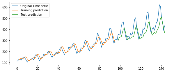
DataPreparationRNN.PintaResultado(dataset,trainPredict,testPredict,look_back)
Train Score: 0.61 RMSE
Test Score: 0.72 RMSE
Train Score: 1.54 MAPE
Test Score: 1.26 MAPE
5
plt.plot(scaler.inverse_transform(y_test.flatten()[:, np.newaxis]),'b',label='Real KO Stock Price')
plt.plot(testPredict.flatten(),'g',label='Predicted KO Stock Price')
plt.legend()
plt.show()
Encoder-Decoder architecture (sequence-to-sequence)#
Input: [n_samples,3,1]
Ouput: [n_samples,3,1]
look_back = 10;
time_ahead = 7
dataset = dataset1.values
dataset = dataset.astype('float32')

# split into train and test sets
test_size = 600
train_size = int(len(dataset) - test_size)
train, test = dataset[0:train_size], dataset[train_size:len(dataset)]

# normalize the dataset
scaler = MinMaxScaler(feature_range=(0, 1))
trainN = scaler.fit_transform(train)
testN = scaler.transform(test)

X_train, y_train = DataPreparationRNN.create_datasetMultipleTimesBackAhead(trainN, n_steps_out=time_ahead, n_steps_in = look_back, overlap = time_ahead)
X_train2, y_train2 = DataPreparationRNN.create_datasetMultipleTimesBackAhead(trainN, n_steps_out=time_ahead, n_steps_in = look_back, overlap = 1)
X_test, y_test = DataPreparationRNN.create_datasetMultipleTimesBackAhead(testN, n_steps_out=time_ahead, n_steps_in = look_back, overlap = time_ahead)

model8b = Sequential()
model8b.add(SimpleRNN(20,activation = 'relu',input_shape=(look_back,1)))
model8b.add(RepeatVector(time_ahead))
model8b.add(SimpleRNN(20,activation = 'relu',return_sequences=True))
model8b.add(TimeDistributed(Dense(1)))


model8b.compile(optimizer='adam',loss='mse')
model8b.fit(X_train2.reshape(X_train2.shape[0],look_back,1),y_train2.reshape(y_train2.shape[0],time_ahead,1),epochs=1000, verbose=0)
trainPredict, testPredict = DataPreparationRNN.EstimaRMSE_RNN_MultiStepEncoDeco(model8b,X_train,X_test,y_train,y_test,scaler,look_back,time_ahead)
DataPreparationRNN.PintaResultado(dataset,trainPredict,testPredict,look_back)
Train Score: 0.56 RMSE
Test Score: 0.89 RMSE
Train Score: 1.28 MAPE
Test Score: 1.59 MAPE
5
plt.plot(scaler.inverse_transform(y_test.flatten()[:, np.newaxis]),'b',label='Real KO Stock Price')
plt.plot(testPredict.flatten(),'g',label='Predicted KO Stock Price')
plt.legend()
plt.show()
many-to-one
model8 = Sequential()
model8.add(SimpleRNN(5,activation = 'relu',return_sequences=True,input_shape=(look_back,1)))
model8.add(SimpleRNN(5,activation = 'relu'))
model8.add(Dense(1))

many-to-many
model8 = Sequential()
model8.add(SimpleRNN(5,activation = 'relu',return_sequences=True,input_shape=(look_back,1)))
model8.add(SimpleRNN(5,activation = 'relu',return_sequences=True))
model8.add(TimeDistributeds(Dense(1)))

seq-to-seq
model8 = Sequential()
model8.add(SimpleRNN(5,activation = 'relu',input_shape=(look_back,1)))
model8.add(RepeatVector(repetitions))
model8.add(SimpleRNN(5,activation = 'relu',return_sequences=True))
model8.add(TimeDistributed(Dense(1)))