
3.1 - Symbolic computing for ML#
!wget -nc --no-cache -O init.py -q https://raw.githubusercontent.com/rramosp/2021.deeplearning/main/content/init.py
import init; init.init(force_download=False);
import sys
import sympy as sy
%load_ext tensorboard
sy.init_printing(use_latex=True)
import tensorflow as tf
tf.__version__
'2.4.0'
Recall the machine learning algorithm design process#
from IPython.display import Image
Image(filename='local/imgs/mldesign.jpg', width=800)
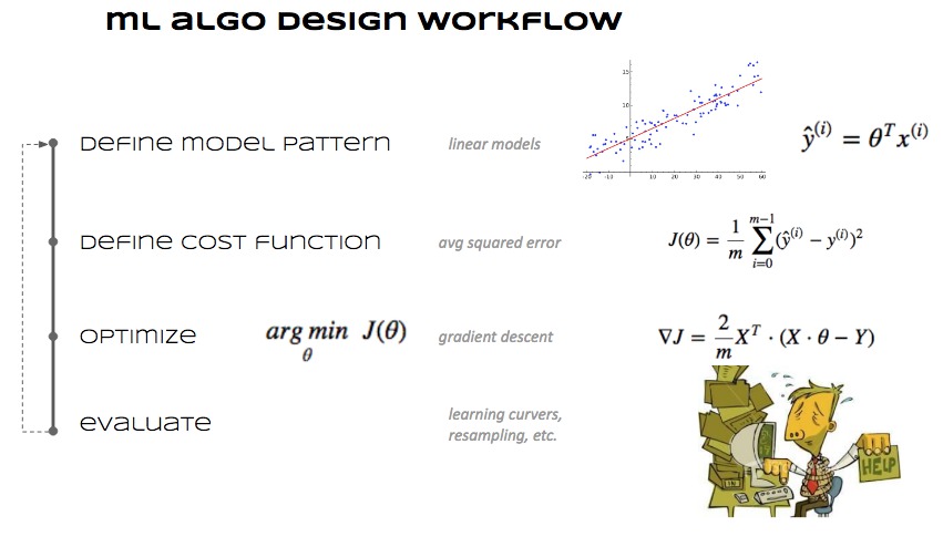
And how we sorted it out for linear regression using a generic optimization library#
Input and expected output (supervised learning)
\(\mathbf{x}^{(i)} \in \mathbb{R}^n\), \(y^{(i)} \in \mathbb{R}\)
Predicción model
\(\hat{y}^{(i)} = \overline{\theta} \dot \; \mathbf{x}^{(i)}\), \(\;\;\;\;\)with \(\overline{\theta} \in \mathbb{R}^n\) and assuming \(\mathbf{x}^{(i)}_0=1\)
Loss function
\(J(\overline{\theta}) = \frac{1}{m} \sum_{i=0}^{m-1}(\overline{\theta} \dot \; \mathbf{x}^{(i)} - y^{(i)})^2\)
Gradient of loss function (matrix form)
\(\nabla J = \begin{bmatrix} \frac{\partial J}{\partial \theta_0}\\ \frac{\partial J}{\partial \theta_1} \end{bmatrix} = \frac{1}{m}2X^{T}\cdot(X\cdot\theta-Y)\)
import numpy as np
import matplotlib.pyplot as plt
import pandas as pd
from scipy.optimize import minimize
%matplotlib inline
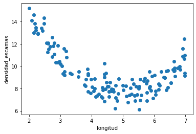
d = pd.read_csv("local/data/trilotropicos.csv")
print(d.shape)
plt.scatter(d.longitud, d.densidad_escamas)
plt.xlabel(d.columns[0])
plt.ylabel(d.columns[1]);
(150, 2)
y = d.densidad_escamas.values
X = np.r_[[[1]*len(d), d.longitud.values]].T


def n_cost(t):
    return np.mean((X.dot(t)-y)**2)

def n_grad(t):
    return 2*X.T.dot(X.dot(t)-y)/len(X)

init_t = np.random.random()*40-5, np.random.random()*20-10
r = minimize(n_cost, init_t, method="BFGS", jac=n_grad)
r
      fun: 2.7447662570806624
 hess_inv: array([[ 5.57455133, -1.09184708],
       [-1.09184708,  0.23443488]])
      jac: array([-1.43724881e-06, -7.18659553e-06])
  message: 'Optimization terminated successfully.'
     nfev: 11
      nit: 10
     njev: 11
   status: 0
  success: True
        x: array([12.68999789, -0.71805919])
Using sympy computer algebra system (CAS)#
x,y = sy.symbols("x y")
z = x**2 + x*sy.cos(y)
z

we can evaluate the expresion by providing concrete values for the symbolic variables
z.subs({x: 2, y: sy.pi/4})

and obtain numerical approximations of these values
sy.N(z.subs({x: 2, y: sy.pi/4}))

a derivative can be seen as a function that inputs and expression and outputs another expression
observe how we compute \(\frac{\partial z}{\partial x}\) and \(\frac{\partial z}{\partial y}\)
z.diff(x)

z.diff(y)

r = z.diff(x).subs({x: 2, y: sy.pi/4})
r, sy.N(r)

r = z.diff(y).subs({x: 2, y: sy.pi/4})
r, sy.N(r)

EXERCISE: draw the computational graph of \(x^2+x\cos(x)\) and show how to differentiate mechanically using the graphs.
More things you can do with sympy (and almost any CAS)
sy.expand((x+2)**2)

sy.factor( x**2-2*x-8 )

sy.solve( x**2 + 2*x - 8, x)

a = sy.symbols("alpha")
sy.solve( a*x**2 + 2*x - 8, x)

differential equations, solving \(\frac{df}{dt}=f(t)+t\)
t, C1 = sy.symbols("t C1")
f = sy.symbols("f", cls=sy.Function)
dydt = f(t)+t
eq = dydt-sy.diff(f(t),t)
yt = sy.dsolve(eq, f(t))
yt

systems of equations
sy.solve ([x**2+y, 3*y-x])

Sympy to Python and Numpy#
f = (sy.sin(x) + x**2)/2
f

f.subs({x:10})

sy.N(f.subs({x:10}))

f1 = sy.lambdify(x, f)
f1(10)
and a vectorized version
f2 = sy.lambdify(x, f, "numpy")
f2(10)
f2(np.array([10,2,3]))
array([49.72798944, 2.45464871, 4.57056 ])
the lambdified version is faster, and the vectorized one is even faster
%timeit sy.N(f.subs({x:10}))
125 µs ± 8.62 µs per loop (mean ± std. dev. of 7 runs, 10000 loops each)
%timeit f1(10)
1.33 µs ± 26.6 ns per loop (mean ± std. dev. of 7 runs, 1000000 loops each)
%timeit [f1(i) for i in range(1000)]
1.38 ms ± 26.7 µs per loop (mean ± std. dev. of 7 runs, 1000 loops each)
%timeit f2(np.arange(1000))
17.6 µs ± 109 ns per loop (mean ± std. dev. of 7 runs, 100000 loops each)
Using sympy to obtain the gradient.#
y = d.densidad_escamas.values
X = np.r_[[[1]*len(d), d.longitud.values]].T

t0,t1 = sy.symbols("theta_0 theta_1")
t0,t1

we first obtain the cost expression for a few summation terms, so that we can print it out and understand it
expr = 0
for i in range(10):
    expr += (X[i,0]*t0+X[i,1]*t1-y[i])**2
expr = expr/len(X)
expr

find X[0] and y[0] in the expression above, beware that you might get simplifications and reordering of the expression by sympy
y[:10]
we can now simplify the expression, using sympy mechanics
expr = expr.simplify()
expr

we now build the full expression
def build_logisitic_regression_cost_expression(X,y):
    expr_cost = 0
    for i in range(len(X)):
        expr_cost += (X[i,0]*t0+X[i,1]*t1-y[i])**2/len(X)
    expr_cost = expr_cost.simplify()
    return expr_cost
y = d.densidad_escamas.values
X = np.r_[[[1]*len(d), d.longitud.values]].T

expr_cost = build_logisitic_regression_cost_expression(X,y)
expr_cost

%timeit build_logisitic_regression_cost_expression(X,y)
2.6 s ± 68.7 ms per loop (mean ± std. dev. of 7 runs, 1 loop each)
obtain derivatives symbolically
expr_dt0 = expr_cost.diff(t0)
expr_dt1 = expr_cost.diff(t1)
expr_dt0, expr_dt1

and obtain regular Python so that we can use them in optimization
s_cost = sy.lambdify([[t0,t1]], expr_cost, "numpy")

d0 = sy.lambdify([[t0,t1]], expr_dt0, "numpy")
d1 = sy.lambdify([[t0,t1]], expr_dt1, "numpy")
s_grad = lambda x: np.array([d0(x), d1(x)])
and now we can minimize
r = minimize(s_cost, [0,0], jac=s_grad, method="BFGS")
r
      fun: 2.7447662570799594
 hess_inv: array([[ 5.57425906, -1.09086733],
       [-1.09086733,  0.23434848]])
      jac: array([-1.73778293e-07, -9.26928138e-07])
  message: 'Optimization terminated successfully.'
     nfev: 10
      nit: 9
     njev: 10
   status: 0
  success: True
        x: array([12.6899981, -0.7180591])
observe that hand derived functions and the ones obtained by sympy evaluate to the same values
t0 = np.random.random()*5+10
t1 = np.random.random()*4-3
t = np.r_[t0,t1]

print ("theta:",t)
print ("cost analytic:", n_cost(t))
print ("cost symbolic:", s_cost(t))

print ("gradient analytic:", n_grad(t))
print ("gradient symbolic:", s_grad(t))
theta: [13.38981165 -1.04706873]
cost analytic: 3.664362725033482
cost symbolic: 3.6643627250332145
gradient analytic: [-1.66013083 -9.12123711]
gradient symbolic: [-1.66013083 -9.12123711]