4.7 - Transposed convolutions#
!wget -nc --no-cache -O init.py -q https://raw.githubusercontent.com/rramosp/2021.deeplearning/main/content/init.py
import init; init.init(force_download=False);
/content/init.py:2: SyntaxWarning: invalid escape sequence '\S'
  course_id = '\S*deeplearning\S*'
replicating local resources
import numpy as np
import tensorflow as tf
import matplotlib.pyplot as plt
import pandas as pd
%matplotlib inline
%load_ext tensorboard
from time import time
tf.__version__
'2.19.0'
Types of convolutions#
See Types of convolutions for a global view of how convolutions can be made in different ways.
Complementary refs:
Architectures:#
Convolution matrix#
we have the following (very small) image and filter
simg = np.r_[[[4,5,8,7],[1,8,8,8],[3,6,6,4],[6,5,7,8]]].astype(np.float32)
akernel = np.r_[[[10,-4,10],[10,4-4,30],[30,30,-1]]]
print ("image\n", simg)
print ("--\nfilter\n", akernel)
image
 [[4. 5. 8. 7.]
 [1. 8. 8. 8.]
 [3. 6. 6. 4.]
 [6. 5. 7. 8.]]
--
filter
 [[10 -4 10]
 [10  0 30]
 [30 30 -1]]
and a VALID convolution (with TF and by hand)
c1 = tf.keras.layers.Conv2D(filters=1, kernel_size=akernel.shape, padding="VALID", activation="linear")
c1.build(input_shape=[None, *simg[:,:,None].shape])
c1.set_weights([akernel[:,:,None, None], np.r_[0]])

routput = c1(simg[None, :, :, None]).numpy()
print(routput[0,:,:,0])
[[614. 764.]
 [591. 660.]]
np.r_[[[(simg[:3,:3]*akernel).sum(), (simg[:3,1:]*akernel).sum()],\
       [(simg[1:,:3]*akernel).sum(), (simg[1:,1:]*akernel).sum()]]]
array([[614., 764.],
       [591., 660.]])
observe we can arrange the filter into a convolutional matrix, so that a .dot operation gets the same result.
with
\(am \in \mathbb{R}^{4}\), that can be reshaped into \(\mathbb{R}^{2\times 2}\)
\(cm \in \mathbb{R}^{4\times 16}\)
\(img \in \mathbb{R}^{16}\), reshaped from \(\mathbb{R}^{4\times 4}\)
cm = np.array([[10., -4., 10.,  0., 10.,  0., 30.,  0., 30., 30., -1.,  0.,  0., 0.,  0.,   0.],
               [ 0., 10., -4., 10.,  0., 10.,  0., 30.,  0., 30., 30., -1.,  0., 0.,  0.,   0.],
               [ 0.,  0.,  0.,  0., 10., -4., 10.,  0., 10.,  0., 30.,  0., 30., 30., -1.,  0.],
               [ 0.,  0.,  0.,  0.,  0., 10., -4., 10.,  0., 10.,  0., 30.,  0., 30., 30., -1.]])

dx, dy = np.r_[simg.shape[0] - akernel.shape[0]+1, simg.shape[1] - akernel.shape[1]+1]
am = cm.dot(simg.flatten()).reshape(dx,dy)
am
array([[614., 764.],
       [591., 660.]])
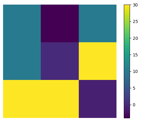
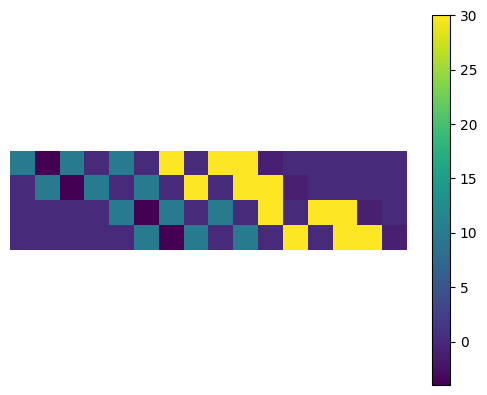
observe that cm is just the same akernel replicated and re-arranged
plt.imshow(akernel); plt.axis("off")
plt.colorbar();
plt.imshow(cm); plt.axis("off")
plt.colorbar();
Transposed convolutions#
we can turn the .dot product around by using cm´s transpose matrix. This IS NOT in general an inverse operation, but the dimensions are kept and can be used to recover reduced dimensions.
with
\(img´ \in \mathbb{R}^{16}\), that can be reshaped from \(\mathbb{R}^{4\times 4}\)
\(cm \in \mathbb{R}^{16\times 4}\)
\(am \in \mathbb{R}^{4}\), reshaped into \(\mathbb{R}^{2\times 2}\)
cm.T.dot(am.flatten()).reshape(simg.shape)
array([[ 6140.,  5184.,  3084.,  7640.],
       [12050., 11876., 21690., 29520.],
       [24330., 47940., 40036., 19036.],
       [17730., 37530., 19209.,  -660.]])
which is implemented as a Conv2DTransposed Keras layer
ct = tf.keras.layers.Conv2DTranspose(filters=1, kernel_size=akernel.shape, activation="linear")
ct.build(input_shape=[None, *am[:,:,None].shape])
ct.set_weights((akernel[:,:, None, None], np.r_[0]))
ct(am[None, :, :, None]).numpy()[0,:,:,0]
array([[ 6140.,  5184.,  3084.,  7640.],
       [12050., 11876., 21690., 29520.],
       [24330., 47940., 40036., 19036.],
       [17730., 37530., 19209.,  -660.]], dtype=float32)
observe how a transposed convolution is simply a convolution with a padded and dilated input img
def dilate(simg):
    k = simg.copy()
    for i in range(k.shape[1]-1):
        k = np.insert(k, 1+2*i, values=0, axis=1)
    for i in range(k.shape[0]-1):
        k = np.insert(k, 1+2*i, values=0, axis=0)
    return k

def pad(am, n):
    k = np.append(am,np.zeros((n,am.shape[1])), axis=0)
    k = np.append(k,np.zeros((k.shape[0],n)), axis=1)
    k = np.append(np.zeros((k.shape[0],n)), k, axis=1)
    k = np.append(np.zeros((n, k.shape[1])), k, axis=0)
    return k
dam = pad(am, 2)
dam
array([[  0.,   0.,   0.,   0.,   0.,   0.],
       [  0.,   0.,   0.,   0.,   0.,   0.],
       [  0.,   0., 614., 764.,   0.,   0.],
       [  0.,   0., 591., 660.,   0.,   0.],
       [  0.,   0.,   0.,   0.,   0.,   0.],
       [  0.,   0.,   0.,   0.,   0.,   0.]])
a transposed convolution implemented with a regular convolution
dkernel = akernel[::-1,::-1] # hacking to conform to TF

c1 = tf.keras.layers.Conv2D(filters=1, kernel_size=dkernel.shape, padding="VALID", activation="linear")
c1.build(input_shape=[None, *simg[:,:,None].shape])
c1.set_weights([dkernel.T[:,:,None, None], np.r_[0]])

routput = c1(dam.T[None, :, :, None]).numpy().T
print(routput[0,:,:,0])
[[ 6140.  5184.  3084.  7640.]
 [12050. 11876. 21690. 29520.]
 [24330. 47940. 40036. 19036.]
 [17730. 37530. 19209.  -660.]]
the same transposed convolution with a Conv2DTranspose layer
ct = tf.keras.layers.Conv2DTranspose(filters=1, kernel_size=akernel.shape, activation="linear")
ct.build(input_shape=[None, *am[:,:,None].shape])
ct.set_weights((akernel[:,:, None, None], np.r_[0]))
ct(am[None, :, :, None]).numpy()[0,:,:,0]
array([[ 6140.,  5184.,  3084.,  7640.],
       [12050., 11876., 21690., 29520.],
       [24330., 47940., 40036., 19036.],
       [17730., 37530., 19209.,  -660.]], dtype=float32)
now with stride (i.e. dilation on the input image)
ct = tf.keras.layers.Conv2DTranspose(filters=1, strides=2, kernel_size=akernel.shape, activation="linear")
ct.build(input_shape=[None, *am[:,:,None].shape])
ct.set_weights((akernel[:,:, None, None], np.r_[0]))
ct(am[None, :, :, None]).numpy()[0,:,:,0]
array([[ 6140., -2456., 13780., -3056.,  7640.],
       [ 6140.,     0., 26060.,     0., 22920.],
       [24330., 16056., 34816., 20280.,  5836.],
       [ 5910.,     0., 24330.,     0., 19800.],
       [17730., 17730., 19209., 19800.,  -660.]], dtype=float32)
which is equivalent to a convolution with dilation on the input image
# the input image with padding and dilation
dam = pad(dilate(am), 2)
dam
array([[  0.,   0.,   0.,   0.,   0.,   0.,   0.],
       [  0.,   0.,   0.,   0.,   0.,   0.,   0.],
       [  0.,   0., 614.,   0., 764.,   0.,   0.],
       [  0.,   0.,   0.,   0.,   0.,   0.,   0.],
       [  0.,   0., 591.,   0., 660.,   0.,   0.],
       [  0.,   0.,   0.,   0.,   0.,   0.,   0.],
       [  0.,   0.,   0.,   0.,   0.,   0.,   0.]])
dkernel = akernel[::-1,::-1] # hacking to conform to TF

c1 = tf.keras.layers.Conv2D(filters=1, kernel_size=dkernel.shape, padding="VALID", activation="linear")
c1.build(input_shape=[None, *simg[:,:,None].shape])
c1.set_weights([dkernel.T[:,:,None, None], np.r_[0]])

routput = c1(dam.T[None, :, :, None]).numpy().T
print(routput[0,:,:,0])
[[ 6140. -2456. 13780. -3056.  7640.]
 [ 6140.     0. 26060.     0. 22920.]
 [24330. 16056. 34816. 20280.  5836.]
 [ 5910.     0. 24330.     0. 19800.]
 [17730. 17730. 19209. 19800.  -660.]]
for curiosity, can we find any \(am\) such that \(img \approx img'\)? Observe how
we set the values of a convolutional filter for which
trainable=Falsewe fit the
Conv2DTransposeparameters so that the output is a similar as possible to the inputwe train with the same input-output values
This is, somehow, like a convolutional autoencoder, where we fix the encoder and what to find out the decoder.
def get_model(img_size=4, compile=True):
    inputs = tf.keras.Input(shape=(img_size,img_size,1), name="input_1")
    layers = tf.keras.layers.Conv2D(1,(3,3), activation="linear", padding="SAME", trainable=False)(inputs)
    outputs = tf.keras.layers.Conv2DTranspose(1,(3,3), strides=1, activation="linear", padding="SAME")(layers)
    model = tf.keras.Model(inputs = inputs, outputs=outputs)
    if compile:
        model.compile(optimizer='adam',
                      loss='mse',
                      metrics=['mse'])
    return model
m = get_model()
m.summary()
Model: "functional"
┏━━━━━━━━━━━━━━━━━━━━━━━━━━━━━━━━━┳━━━━━━━━━━━━━━━━━━━━━━━━┳━━━━━━━━━━━━━━━┓
┃ Layer (type)                    ┃ Output Shape           ┃       Param # ┃
┡━━━━━━━━━━━━━━━━━━━━━━━━━━━━━━━━━╇━━━━━━━━━━━━━━━━━━━━━━━━╇━━━━━━━━━━━━━━━┩
│ input_1 (InputLayer)            │ (None, 4, 4, 1)        │             0 │
├─────────────────────────────────┼────────────────────────┼───────────────┤
│ conv2d_4 (Conv2D)               │ (None, 4, 4, 1)        │            10 │
├─────────────────────────────────┼────────────────────────┼───────────────┤
│ conv2d_transpose_4              │ (None, 4, 4, 1)        │            10 │
│ (Conv2DTranspose)               │                        │               │
└─────────────────────────────────┴────────────────────────┴───────────────┘
Total params: 20 (80.00 B)
Trainable params: 10 (40.00 B)
Non-trainable params: 10 (40.00 B)
m.build(input_shape=[None, *am[:,:,None].shape])
m.layers[1].set_weights((akernel[:,:, None, None], np.r_[0]))
m.fit(simg[None, :,:, None], simg[None, :,:, None], epochs=10000, verbose=False)
<keras.src.callbacks.history.History at 0x79c5944704d0>
observe that the reconstructed image values are somewhat similar to the input image
m(simg[None, :,:, None])[0,:,:,0].numpy()
array([[3.6894827, 4.0357714, 6.010421 , 7.1442747],
       [2.2414048, 7.59128  , 8.780073 , 7.7545385],
       [3.7473285, 6.9444914, 8.552898 , 4.787974 ],
       [4.658065 , 3.4127903, 4.7543545, 6.9866705]], dtype=float32)
simg
array([[4., 5., 8., 7.],
       [1., 8., 8., 8.],
       [3., 6., 6., 4.],
       [6., 5., 7., 8.]], dtype=float32)
these two filters try to be convolutional inverses of each other (this is not a rigorous definition, just an intuition!!)
m.layers[1].get_weights()[0][:,:,0,0]
array([[10., -4., 10.],
       [10.,  0., 30.],
       [30., 30., -1.]], dtype=float32)
m.layers[2].get_weights()[0][:,:,0,0]
array([[ 0.00405932, -0.00111854, -0.00293583],
       [ 0.00037578, -0.00354484,  0.01345906],
       [-0.00630359,  0.0161382 , -0.01294528]], dtype=float32)
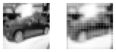
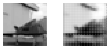
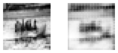
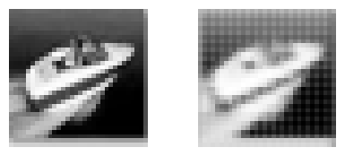
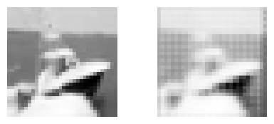
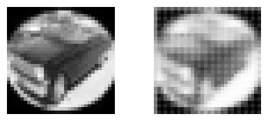
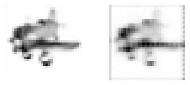
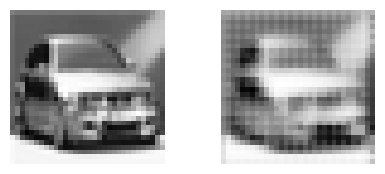
Downsampling and upsampling#
we use our mini_cifar, observe how:
the following models downsize and then upsize the input.
input and output shapes of the models are the same
we set up a loss function to reconstruct the input in the output.
the reconstruction quality with
modelAwithn_filters=1andn_filters=10, and withmodelB.the artifacts that reconstruction generates.
import h5py
!wget -nc -q https://s3.amazonaws.com/rlx/mini_cifar.h5
with h5py.File('mini_cifar.h5','r') as h5f:
    x_cifar = h5f["x"][:][:1000]
    y_cifar = h5f["y"][:][:1000]
x_cifar = x_cifar.mean(axis=3)[:,:,:,None] # observe we convert cifar to grayscale
x_cifar.shape, y_cifar.shape
((1000, 32, 32, 1), (1000,))
model A reduces the activation map dimensions with a MaxPool2D layer. It only has one Conv2D layer
def get_modelA(img_size=32, compile=True):
    inputs = tf.keras.Input(shape=(img_size,img_size,1), name="input_1")
    layers = tf.keras.layers.Conv2D(20,(3,3), activation="tanh", padding="SAME", trainable=False)(inputs)
    layers = tf.keras.layers.MaxPool2D(2)(layers)
    outputs = tf.keras.layers.Conv2DTranspose(1,(3,3), strides=2, activation="tanh", padding="SAME")(layers)
    model = tf.keras.Model(inputs = inputs, outputs=outputs)
    if compile:
        model.compile(optimizer='adam',
                      loss='mse',
                      metrics=['mse'])
    return model
model B reduces the activation map dimensions with a stride=2 on the convolutional layer. It also has 2 Conv2D layers
def get_modelB(img_size=32, compile=True):
    inputs = tf.keras.Input(shape=(img_size,img_size,1), name="input_1")
    layers = tf.keras.layers.Conv2D(5,(3,3), activation="tanh", padding="SAME", trainable=False)(inputs)
    layers = tf.keras.layers.Conv2D(15,(3,3), strides=2, activation="sigmoid", padding="SAME", trainable=False)(inputs)
    outputs = tf.keras.layers.Conv2DTranspose(1,(3,3), strides=2, activation="tanh", padding="SAME")(layers)
    model = tf.keras.Model(inputs = inputs, outputs=outputs)
    if compile:
        model.compile(optimizer='adam',
                      loss='mse',
                      metrics=['mse'])
    return model
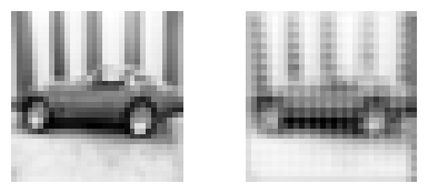
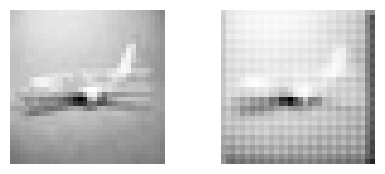
observe the different artifacts created in each case
#m = get_modelA()
m = get_modelB()
m.summary()
Model: "functional_1"
┏━━━━━━━━━━━━━━━━━━━━━━━━━━━━━━━━━┳━━━━━━━━━━━━━━━━━━━━━━━━┳━━━━━━━━━━━━━━━┓
┃ Layer (type)                    ┃ Output Shape           ┃       Param # ┃
┡━━━━━━━━━━━━━━━━━━━━━━━━━━━━━━━━━╇━━━━━━━━━━━━━━━━━━━━━━━━╇━━━━━━━━━━━━━━━┩
│ input_1 (InputLayer)            │ (None, 32, 32, 1)      │             0 │
├─────────────────────────────────┼────────────────────────┼───────────────┤
│ conv2d_6 (Conv2D)               │ (None, 16, 16, 15)     │           150 │
├─────────────────────────────────┼────────────────────────┼───────────────┤
│ conv2d_transpose_5              │ (None, 32, 32, 1)      │           136 │
│ (Conv2DTranspose)               │                        │               │
└─────────────────────────────────┴────────────────────────┴───────────────┘
Total params: 286 (1.12 KB)
Trainable params: 136 (544.00 B)
Non-trainable params: 150 (600.00 B)
m.fit(x_cifar, x_cifar, epochs=20, batch_size=1)
Epoch 1/20
1000/1000 ━━━━━━━━━━━━━━━━━━━━ 2s 2ms/step - loss: 0.0847 - mse: 0.0847
Epoch 2/20
1000/1000 ━━━━━━━━━━━━━━━━━━━━ 2s 2ms/step - loss: 0.0463 - mse: 0.0463
Epoch 3/20
1000/1000 ━━━━━━━━━━━━━━━━━━━━ 2s 2ms/step - loss: 0.0368 - mse: 0.0368
Epoch 4/20
1000/1000 ━━━━━━━━━━━━━━━━━━━━ 3s 2ms/step - loss: 0.0298 - mse: 0.0298
Epoch 5/20
1000/1000 ━━━━━━━━━━━━━━━━━━━━ 2s 2ms/step - loss: 0.0238 - mse: 0.0238
Epoch 6/20
1000/1000 ━━━━━━━━━━━━━━━━━━━━ 2s 2ms/step - loss: 0.0197 - mse: 0.0197
Epoch 7/20
1000/1000 ━━━━━━━━━━━━━━━━━━━━ 3s 2ms/step - loss: 0.0164 - mse: 0.0164
Epoch 8/20
1000/1000 ━━━━━━━━━━━━━━━━━━━━ 3s 2ms/step - loss: 0.0143 - mse: 0.0143
Epoch 9/20
1000/1000 ━━━━━━━━━━━━━━━━━━━━ 2s 2ms/step - loss: 0.0127 - mse: 0.0127
Epoch 10/20
1000/1000 ━━━━━━━━━━━━━━━━━━━━ 2s 2ms/step - loss: 0.0114 - mse: 0.0114
Epoch 11/20
1000/1000 ━━━━━━━━━━━━━━━━━━━━ 2s 2ms/step - loss: 0.0099 - mse: 0.0099
Epoch 12/20
1000/1000 ━━━━━━━━━━━━━━━━━━━━ 3s 2ms/step - loss: 0.0097 - mse: 0.0097
Epoch 13/20
1000/1000 ━━━━━━━━━━━━━━━━━━━━ 2s 2ms/step - loss: 0.0092 - mse: 0.0092
Epoch 14/20
1000/1000 ━━━━━━━━━━━━━━━━━━━━ 2s 2ms/step - loss: 0.0084 - mse: 0.0084
Epoch 15/20
1000/1000 ━━━━━━━━━━━━━━━━━━━━ 2s 2ms/step - loss: 0.0080 - mse: 0.0080
Epoch 16/20
1000/1000 ━━━━━━━━━━━━━━━━━━━━ 2s 2ms/step - loss: 0.0077 - mse: 0.0077
Epoch 17/20
1000/1000 ━━━━━━━━━━━━━━━━━━━━ 2s 2ms/step - loss: 0.0071 - mse: 0.0071
Epoch 18/20
1000/1000 ━━━━━━━━━━━━━━━━━━━━ 3s 2ms/step - loss: 0.0068 - mse: 0.0068
Epoch 19/20
1000/1000 ━━━━━━━━━━━━━━━━━━━━ 2s 2ms/step - loss: 0.0068 - mse: 0.0068
Epoch 20/20
1000/1000 ━━━━━━━━━━━━━━━━━━━━ 3s 2ms/step - loss: 0.0067 - mse: 0.0067
<keras.src.callbacks.history.History at 0x79c594472fc0>
px_cifar = m.predict(x_cifar)
32/32 ━━━━━━━━━━━━━━━━━━━━ 0s 8ms/step
for _ in range(10):
    i = np.random.randint(len(x_cifar))
    plt.figure(figsize=(5,2))
    plt.subplot(121); plt.imshow(x_cifar[i,:,:,0], cmap=plt.cm.Greys_r); plt.axis("off")
    plt.subplot(122); plt.imshow(px_cifar[i,:,:,0], cmap=plt.cm.Greys_r); plt.axis("off")