
LAB 2.2 - Sparse Autoencoders#
!wget -nc --no-cache -O init.py -q https://raw.githubusercontent.com/rramosp/2021.deeplearning/main/content/init.py
import init; init.init(force_download=False); init.get_weblink()
from local.lib.rlxmoocapi import submit, session
import inspect
session.LoginSequence(endpoint=init.endpoint, course_id=init.course_id, lab_id="L02.02", varname="student");
LAB SUMMARY#
In this lab we will create a Sparse Autoencoder, where we will force the encoder to have SMALL ACTIVATIONS. we will continue to use MNIST
import numpy as np
import matplotlib.pyplot as plt
import pandas as pd

from keras import Sequential, Model
from keras.layers import Dense, Dropout, Flatten, Input
from keras.losses import Loss
import tensorflow as tf

%matplotlib inline
mnist = pd.read_csv("local/data/mnist1.5k.csv.gz", compression="gzip", header=None).values
X=(mnist[:,1:785]/255.).astype(np.float32)
y=(mnist[:,0]).astype(int)
print("dimension de las imagenes y las clases", X.shape, y.shape)
from sklearn.model_selection import train_test_split
X_train, X_test, y_train, y_test = train_test_split(X, y, test_size=.2)
print (X_train.shape, y_train.shape, X_test.shape, y_test.shape)
TASK 01: Handcrafted sparse autoencoder#
Given:
input \(X_{in} \in \mathbb{R}^{m\times n}\) = \(\{ x^{(0)}, x^{(1)},..., x^{(m-1)} \}\), with \(x^{(i)} \in \mathbb{R}^n\)
encoder weights and bias: \(W_e \in \mathbb{R}^{n \times c}\), \(b_e \in \mathbb{R}^{c}\)
decoder weights and bias: \(W_d \in \mathbb{R}^{c \times n}\), \(b_d \in \mathbb{R}^{n}\)
with:
\(n\) the input data dimension
\(m\) the number of input data items
\(c\) the autoencoder
code_size
An autoencoder output is computed as a regular neural network
where:
\(X_{out} \in \mathbb{R}^{m\times n}\) is the output
\(d(X) = \sigma(X \times W_d + b_d)\) is the decoder function
\(e(X) = \text{r}(X \times W_e + b_e)\) is the encoder function
\(\sigma(z) = 1/(1+e^{-z})\) is the sigmoid activation function
\(r(z) = \text{max}(0, z)\) is the ReLU activation function
and we use the following loss function
observe that:
we pretend to penalize large values of the encoder activations, with \(\beta\) regulating how much we penalize
as we are using ReLU there is no need to square \(e(x^{(i)})\)
the summations are over the number of elements (\(m\), with the running index \(i \in [0,..,m-1]\)) and the number of columns (\(n\) for the first term, \(c\) for the second term)
Complete the following function to compute the encoder output and loss. All arguments are numpy arrays. The Xout output must also be a numpy array and loss must be a number. You cannot use Tensorflow to implement your function.
def apply_autoencoder(Xin, We, be, Wd, bd, beta=0.05):

    sigm = lambda z: 1/(1+np.exp(-z))
    relu = lambda z: z*(z>0)

    Xout = ...
    loss = ...

    return Xout, loss
test your code
#
# --- you should get the following output up to three decimals ---
#
# Xout
#  [[0.53992624 0.54127547 0.40167658 0.59832582]
#  [0.580101   0.55012488 0.42321322 0.59509962]
#  [0.62155216 0.52174768 0.43006826 0.62407879]
#  [0.55635373 0.54059637 0.40857522 0.60072369]
#  [0.62178687 0.51694816 0.42812613 0.62813387]]
# loss
#  0.5723349282191469

Xin = np.array([[-0.37035694, -0.34542735,  0.15605706, -0.33053004],
                [-0.3153002 , -0.41249585,  0.30073246,  0.13771319],
                [-0.30017424, -0.15409659, -0.43102843,  0.38578104],
                [-0.14914677, -0.4411987 , -0.33116959, -0.32483895],
                [-0.17407847,  0.0946155 , -0.48391975,  0.34075492]])

We = np.array([[-0.28030543, -0.46140969, -0.18068483],
               [ 0.31530074,  0.29354581, -0.30835241],
               [-0.35849794, -0.12389752, -0.01763293],
               [ 0.44245022, -0.4465276 , -0.40293482]])

be = np.array([ 0.33030961,  0.33221543, -0.32828997])

Wd = np.array([[ 0.42964391, -0.22892199,  0.09340045,  0.25372971],
               [-0.41209546, -0.23107885, -0.28591832,  0.15998353],
               [-0.16731707, -0.10630373, -0.15786946, -0.20899463]])

bd = np.array([ 0.32558449,  0.31610265, -0.25844944,  0.28249571])

Xout, loss = apply_autoencoder(Xin, We, be, Wd, bd)

print ("Xout\n", Xout)
print ("loss\n", loss)
Try your code with other cases
n,m,c = 4, 5, 3

Xin = np.random.random(size=(m,n))-.5
We  = np.random.random(size=(n,c))-.5
be  = np.random.random(size=c)-.5

Wd  = np.random.random(size=(c,n))-.5
bd  = np.random.random(size=n)-.5

Xout, loss = apply_autoencoder(Xin, We, be, Wd, bd)

print ("Xout\n", Xout)
print ("loss\n", loss)
Registra tu solución en linea
student.submit_task(namespace=globals(), task_id='T1');
TASK 02: Sparse autoencoder model#
Complete the get_model function so that the returned model uses the loss function previously defined.
Using the UNSUPERVISED method to specify your loss function, as described in the notes, requires defining the model through the subclassing method. To simplify the implementation, we will use a standard supervised model where input and target correspond to the same tensor. To specify the loss function, two parts MUST be completed:
The regularization term must be added to the encoder layer using aactivity_regularizer. Note that you can add a custom function.
The reconstruction error must be added to the compile method. You can use the default
mseor implement it on your own by subclassing the class Loss keras.
Note for models you have to use Tensorflow operations in specific you have to use tf.reduce_mean or keras operations ops.mean
def get_model(input_dim, code_size, beta=.01):
    from keras import Sequential, Model
    from keras.layers import Dense, Dropout, Flatten, Input
    import tensorflow as tf

    inputs = Input(shape=input_dim, name="input")
    encoder = Dense(code_size, activation='relu', name="encoder",
                    activity_regularizer=...)(inputs)
    outputs = Dense(input_dim, activation='sigmoid', name="decoder")(encoder)

    #class Sparse_AE_loss(Loss):
    #  def call(self, inputs, outputs):
    #      return ...

    model = Model([inputs], [outputs])


    model.compile(loss=...,optimizer='adam')
    return model
to manually check your code verify that you get the same results with your model and with the function from previous exercise. Observe the possible difference in number precisions (32 vs 64 bits)
# output and loss from TF model in this task
def get_loss(model, Xinput):
    return model.evaluate(Xinput, Xinput, verbose=0)

model = get_model(input_dim=X.shape[1], code_size=50, beta=0.05)
print (model(X_train).numpy())
print (get_loss(model, X_train))
# output and loss from previous task
We, be, Wd, wd = model.get_weights()
Xout, loss = apply_autoencoder(X_train, We, be, Wd, wd, beta=0.05)
print(Xout)
print(loss)
you can now train the autoencoder and check its behavior
model.fit(X_train, X_train, epochs=100, batch_size=32)
test the reconstruction#
X_sample = np.random.permutation(X_test)[:10]
X_pred   = model.predict(X_sample)

plt.figure(figsize=(20,5))
for i in range(len(X_sample)):
    plt.subplot(2,len(X_sample),i+1)
    plt.imshow(X_sample[i].reshape(28,28), cmap=plt.cm.Greys_r)
    plt.axis("off")
    plt.subplot(2,len(X_sample),len(X_sample)+i+1)
    plt.imshow(X_pred[i].reshape(28,28), cmap=plt.cm.Greys_r)
    plt.axis("off")
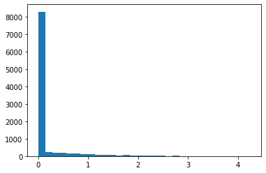
In a similar fashion to the corresponding course notes, you can inspect the encoder and decoder weights, and also the activations and distributions in the latent space.
For activations, you should get something similar to this, indicating a much more sparse representation
from IPython.display import Image
Image("local/imgs/ae_sparse_activations.png")
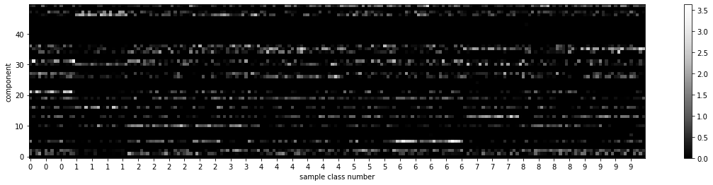
indicating most activations are now very close to zero
Image("local/imgs/ae_activations_distribution.png")
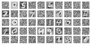
And you should see some latent neurons got specialized when inspecting the decoder weights
Image("local/imgs/decoder_weights.png")
def show_img_grid(w):
    plt.figure(figsize=(10,10))
    for k,wi in enumerate(w):
        plt.subplot(10,10,k+1)
        plt.imshow(wi.reshape(28,28), cmap=plt.cm.Greys_r)
        plt.axis("off")
Registra tu solución en linea
student.submit_task(namespace=globals(), task_id='T2');