4.6 - Object detection

!wget -nc --no-cache -O init.py -q https://raw.githubusercontent.com/rramosp/2021.deeplearning/main/content/init.py
import init; init.init(force_download=False); 

import numpy as np
import tensorflow as tf
import matplotlib.pyplot as plt
import pandas as pd
%matplotlib inline
%load_ext tensorboard

from sklearn.datasets import *
from local.lib import mlutils
from IPython.display import Image
from skimage import io
tf.__version__

The tensorboard extension is already loaded. To reload it, use:
  %reload_ext tensorboard

'2.4.1'

Object detection

• see the original papers on Yolov3, RetinaNet

Approaches:

• Classical: Sliding window, costly

• Two Stage Detectors: First obtain proposed regions, then classify.

• One Stage Detectors: Use region priors on fixed image grid

Observe how an image is annotated for detection

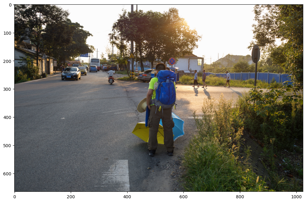
This is an example from the Open Images V6 Dataset, a dataset created and curated at Google. Explore and inspect images and annotations to understand the dataset.

Particularly:

• get a view on the volumetry and class descriptions in https://storage.googleapis.com/openimages/web/factsfigures.html

• understand the image annotation formats in https://storage.googleapis.com/openimages/web/download.html

We download the class descriptions

!wget -nc https://storage.googleapis.com/openimages/v5/class-descriptions-boxable.csv
c = pd.read_csv("class-descriptions-boxable.csv", names=["code", "description"], index_col="code")
c.head()

--2021-01-27 21:15:00--  https://storage.googleapis.com/openimages/v5/class-descriptions-boxable.csv
Resolving storage.googleapis.com (storage.googleapis.com)... 172.217.173.48, 142.250.78.48, 142.250.78.16, ...
Connecting to storage.googleapis.com (storage.googleapis.com)|172.217.173.48|:443... connected.
HTTP request sent, awaiting response... 200 OK
Length: 12011 (12K) [text/csv]
Saving to: ‘class-descriptions-boxable.csv’

class-descriptions- 100%[===================>]  11,73K  --.-KB/s    in 0,002s  

2021-01-27 21:15:01 (6,82 MB/s) - ‘class-descriptions-boxable.csv’ saved [12011/12011]

	description
code
/m/011k07	Tortoise
/m/011q46kg	Container
/m/012074	Magpie
/m/0120dh	Sea turtle
/m/01226z	Football

An example image

img = io.imread("local/imgs/0003bb040a62c86f.jpg")
plt.figure(figsize=(12,10))
plt.imshow(img)

<matplotlib.image.AxesImage at 0x7fa1c5eb8dc0>

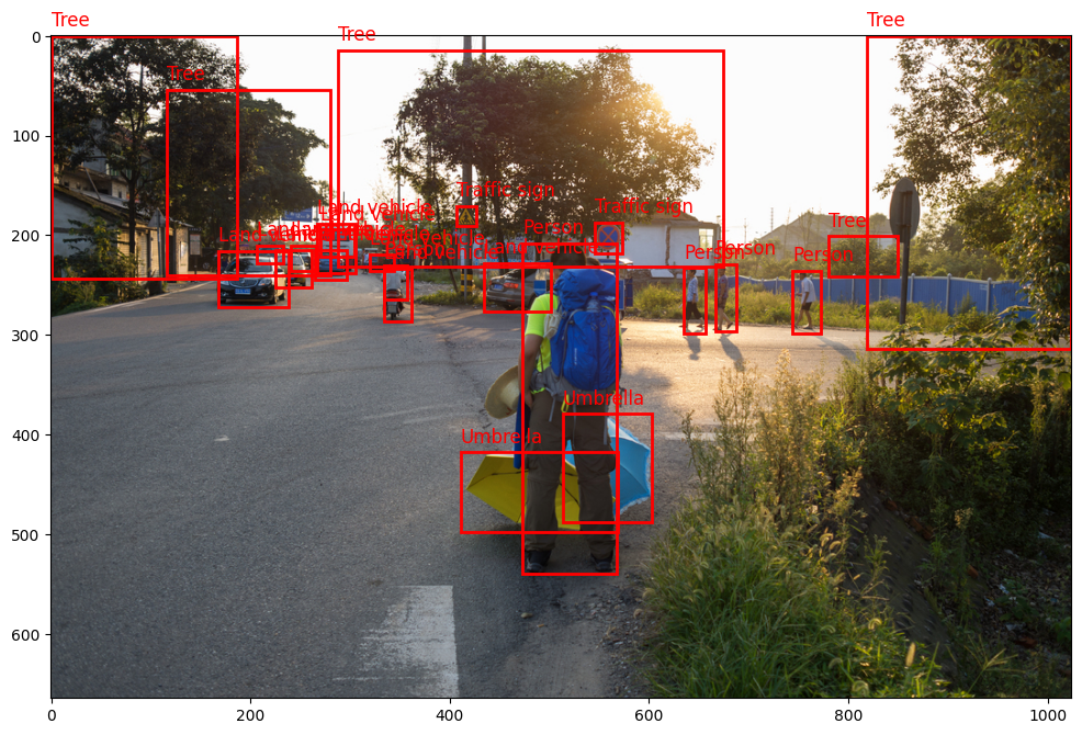
with its annotations

boxes = pd.read_csv("local/data/openimages_boxes_0003bb040a62c86f.csv")
boxes

	ImageID	Source	LabelName	Confidence	XMin	XMax	YMin	YMax	IsOccluded	IsTruncated	...	IsDepiction	IsInside	XClick1X	XClick2X	XClick3X	XClick4X	XClick1Y	XClick2Y	XClick3Y	XClick4Y
0	0003bb040a62c86f	activemil	/m/07j7r	1	0.280625	0.658125	0.021174	0.347449	1	1	...	0	0	-1.000000	-1.000000	-1.000000	-1.000000	-1.000000	-1.000000	-1.000000	-1.000000
1	0003bb040a62c86f	xclick	/m/01g317	1	0.326250	0.349375	0.346487	0.397498	0	0	...	0	0	0.336875	0.326250	0.349375	0.344375	0.346487	0.363811	0.363811	0.397498
2	0003bb040a62c86f	xclick	/m/01g317	1	0.461875	0.553750	0.312801	0.811357	1	0	...	0	0	0.505000	0.461875	0.543750	0.553750	0.312801	0.762271	0.811357	0.760346
3	0003bb040a62c86f	xclick	/m/01g317	1	0.620000	0.641875	0.350337	0.448508	0	0	...	0	0	0.630000	0.620000	0.641875	0.621250	0.350337	0.436959	0.436959	0.448508
4	0003bb040a62c86f	xclick	/m/01g317	1	0.650625	0.671250	0.344562	0.446583	0	0	...	0	0	0.660625	0.650625	0.671250	0.668750	0.344562	0.446583	0.435034	0.442733
5	0003bb040a62c86f	xclick	/m/01g317	1	0.726250	0.754375	0.354187	0.448508	0	0	...	0	0	0.733750	0.726250	0.741250	0.754375	0.354187	0.433109	0.448508	0.401347
6	0003bb040a62c86f	xclick	/m/01mqdt	1	0.397500	0.416875	0.256978	0.286814	0	0	...	0	0	0.397500	0.406250	0.416875	0.416875	0.281039	0.256978	0.286814	0.286814
7	0003bb040a62c86f	xclick	/m/01mqdt	1	0.533125	0.560000	0.281039	0.328200	0	0	...	0	0	0.533125	0.545000	0.560000	0.546250	0.308951	0.281039	0.305101	0.328200
8	0003bb040a62c86f	xclick	/m/01prls	1	0.163750	0.233125	0.325313	0.409047	0	0	...	0	0	0.203750	0.163750	0.218125	0.233125	0.325313	0.379211	0.409047	0.366699
9	0003bb040a62c86f	xclick	/m/01prls	1	0.201875	0.227500	0.316651	0.342637	1	0	...	0	0	0.205625	0.201875	0.218125	0.227500	0.316651	0.332050	0.342637	0.324350
10	0003bb040a62c86f	xclick	/m/01prls	1	0.219375	0.255625	0.323388	0.380173	1	0	...	0	0	0.228750	0.219375	0.249375	0.255625	0.323388	0.336862	0.380173	0.348412
11	0003bb040a62c86f	xclick	/m/01prls	1	0.235000	0.259375	0.316651	0.354187	1	0	...	0	0	0.249375	0.235000	0.254375	0.259375	0.316651	0.326275	0.354187	0.337825
12	0003bb040a62c86f	xclick	/m/01prls	1	0.258125	0.289375	0.323388	0.368624	1	0	...	0	0	0.268750	0.258125	0.282500	0.289375	0.323388	0.331088	0.368624	0.349374
13	0003bb040a62c86f	xclick	/m/01prls	1	0.260625	0.298750	0.282964	0.358037	1	0	...	0	0	0.273125	0.260625	0.293750	0.298750	0.282964	0.305101	0.358037	0.330125
14	0003bb040a62c86f	xclick	/m/01prls	1	0.264375	0.297500	0.292589	0.333975	1	0	...	0	0	0.285000	0.297500	0.297500	0.264375	0.292589	0.333975	0.314726	0.312801
15	0003bb040a62c86f	xclick	/m/01prls	1	0.311875	0.336250	0.330125	0.354187	1	0	...	0	0	0.315625	0.316875	0.311875	0.336250	0.330125	0.354187	0.354187	0.342637
16	0003bb040a62c86f	xclick	/m/01prls	1	0.326250	0.353125	0.351299	0.430221	1	0	...	0	0	0.348125	0.326250	0.339375	0.353125	0.351299	0.390760	0.430221	0.366699
17	0003bb040a62c86f	xclick	/m/01prls	1	0.424375	0.490000	0.342637	0.415784	1	0	...	0	0	0.466875	0.424375	0.468125	0.490000	0.342637	0.391723	0.415784	0.348412
18	0003bb040a62c86f	xclick	/m/07j7r	1	0.000000	0.181875	0.000000	0.366699	1	1	...	0	0	0.071250	0.000000	0.078125	0.181875	0.000000	0.223292	0.366699	0.063523
19	0003bb040a62c86f	xclick	/m/07j7r	1	0.113750	0.273750	0.080847	0.360924	0	0	...	0	0	0.113750	0.188125	0.273750	0.172500	0.210780	0.080847	0.232916	0.360924
20	0003bb040a62c86f	xclick	/m/07j7r	1	0.761875	0.830000	0.302214	0.362849	0	0	...	0	0	0.761875	0.782500	0.830000	0.816250	0.335900	0.302214	0.333013	0.362849
21	0003bb040a62c86f	xclick	/m/07j7r	1	0.799375	0.999375	0.000000	0.471607	0	1	...	0	0	0.799375	0.999375	0.999375	0.999375	0.223292	0.000000	0.461983	0.471607
22	0003bb040a62c86f	xclick	/m/0hnnb	1	0.401250	0.555000	0.628489	0.748797	1	0	...	0	0	0.453750	0.401250	0.519375	0.555000	0.628489	0.681424	0.748797	0.703561
23	0003bb040a62c86f	xclick	/m/0hnnb	1	0.501250	0.588125	0.570741	0.734360	1	0	...	0	0	0.550000	0.501250	0.551250	0.588125	0.570741	0.628489	0.734360	0.697786

24 rows × 21 columns

the annotations of this image

pd.Series([c.loc[i].description for i in boxes.LabelName]).value_counts()

Land vehicle    10
Person           5
Tree             5
Traffic sign     2
Umbrella         2
dtype: int64

from matplotlib.patches import Rectangle
i = np.random.randint(len(boxes))
plt.figure(figsize=(12,10)); 
ax = plt.subplot(111)
plt.imshow(img)
h,w = img.shape[:2]
for i in range(len(boxes)):
    k = boxes.iloc[i]
    label = c.loc[k.LabelName].values[0]
    ax.add_patch(Rectangle((k.XMin*w,k.YMin*h),(k.XMax-k.XMin)*w,(k.YMax-k.YMin)*h, linewidth=2,edgecolor='r',facecolor='none'))
    plt.text(k.XMin*w, k.YMin*h-10, label, fontsize=12, color="red")

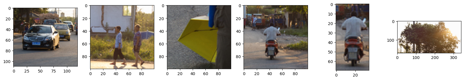
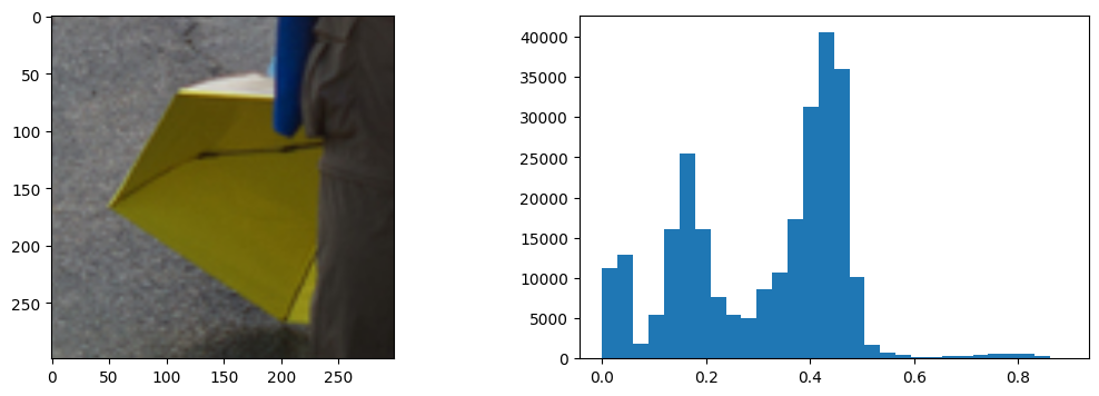
Patch classification, with InceptionV3 from Keras

some sample patches

patches = [img[190:300, 150:270], 
           img[200:300, 600:700], 
           img[400:500, 400:500],
           img[200:300, 300:400],
           img[220:290, 325:360],
           img[10:180, 330:670]]

plt.figure(figsize=(20,3))
for i,pimg in enumerate(patches):
    plt.subplot(1,len(patches),i+1); plt.imshow(pimg)

from tensorflow.keras.applications import inception_v3
if not "model" in locals():
    model = inception_v3.InceptionV3(weights='imagenet', include_top=True)

Downloading data from https://storage.googleapis.com/tensorflow/keras-applications/inception_v3/inception_v3_weights_tf_dim_ordering_tf_kernels.h5
96116736/96112376 [==============================] - 33s 0us/step

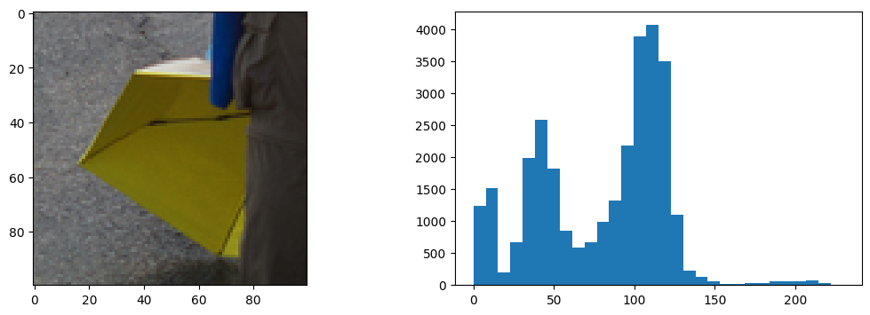
def plot_img_with_histogram(img):
    plt.figure(figsize=(13,4))
    plt.subplot(121)
    plt.imshow(img, vmin=np.min(img), vmax=np.max(img))
    plt.subplot(122)
    plt.hist(img.flatten(), bins=30);

pimg = patches[2]

plot_img_with_histogram(pimg)

from skimage.transform import resize
rimg = resize(pimg, output_shape=(299,299,3))
plot_img_with_histogram(rimg)

pred = model.predict(rimg.reshape(-1,*rimg.shape))
pred.shape

(1, 1000)

k = pd.DataFrame(inception_v3.decode_predictions(pred, top=100)[0], columns=["code", "label", "preds"])
k = k.sort_values(by="preds", ascending=False)

Downloading data from https://storage.googleapis.com/download.tensorflow.org/data/imagenet_class_index.json
40960/35363 [==================================] - 0s 1us/step

plt.figure(figsize=(15,3))
n = 40
plt.bar(range(n), k[:n].preds.values)
plt.xticks(range(n), k[:n].label.values, rotation="vertical");
plt.title("classes with highest prediction probability")
plt.grid();

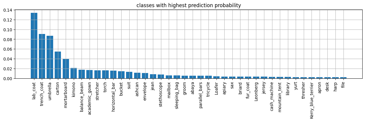
observe how we decode prediction classes. We would nee to align them with our detectiond dataset.

print ('Predicted:')
k = inception_v3.decode_predictions(pred, top=10)[0]
for i in k:
    print("%10s %20s %.6f"%i)

Predicted:
 n03630383             lab_coat 0.134186
 n04479046          trench_coat 0.090892
 n04507155             umbrella 0.087079
 n02971356               carton 0.054701
 n03787032          mortarboard 0.039948
 n03617480               kimono 0.021387
 n02777292         balance_beam 0.017429
 n02669723        academic_gown 0.016952
 n04336792            stretcher 0.016528
 n04456115                torch 0.016192

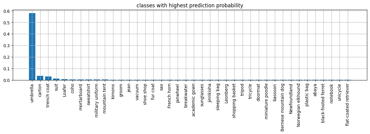
Patch classification, with ResNet model published on TensorFlow Hub

import tensorflow_hub as hub

classnames = pd.read_csv('https://storage.googleapis.com/download.tensorflow.org/data/ImageNetLabels.txt', names=["label"])
if not 'm' in locals():
    m = tf.keras.Sequential([
        hub.KerasLayer("https://tfhub.dev/google/imagenet/inception_resnet_v2/classification/4")
    ])
    m.build([None, 299, 299, 3])  

m.summary()

Model: "sequential"
_________________________________________________________________
Layer (type)                 Output Shape              Param #   
=================================================================
keras_layer (KerasLayer)     (None, 1001)              55875273  
=================================================================
Total params: 55,875,273
Trainable params: 0
Non-trainable params: 55,875,273
_________________________________________________________________

preds = m(rimg.reshape(-1,*rimg.shape).astype(np.float32)).numpy()[0]
preds = np.exp(preds)/np.sum(np.exp(preds))
np.sum(preds)

1.0000002

names = classnames.copy()
names["preds"] = preds
names = names.sort_values(by="preds", ascending=False)
names.head()

	label	preds
880	umbrella	0.581176
479	carton	0.035877
870	trench coat	0.031472
835	suit	0.010810
631	Loafer	0.005403

plt.figure(figsize=(15,3))
n = 40
plt.bar(range(n), names[:n].preds.values)
plt.xticks(range(n), names[:n].label.values, rotation="vertical");
plt.title("classes with highest prediction probability")
plt.grid();

One stage detectors

This blog: YOLO v3 theory explained contains a detailed explanation on how YOLOv3 builds a prediction for detections.

Region priors

A set of box shapes representative of what appears in the training dataset. Obtained typically with KMeans, one must decide how many. For instance

Image("local/imgs/anchor_boxes.png", width=300)

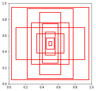
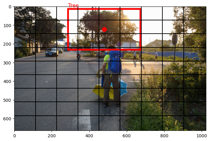
Image fixed partition

• each fixed size image cell is responsible for predicting objects whose center falls within that cell.

• for instance the red dot below signals the tree center and thus the cell responsible for its prediction.

fig = plt.figure(figsize=(8,8))
ax = plt.subplot(111)
plt.imshow(img)
n = 9
for i in range(n):
    plt.axvline(img.shape[1]//n*i, color="black")
    plt.axhline(img.shape[0]//n*i, color="black")
    
k = boxes.iloc[0]
label = c.loc[k.LabelName].values[0]
ax.add_patch(Rectangle((k.XMin*w,k.YMin*h),(k.XMax-k.XMin)*w,(k.YMax-k.YMin)*h, 
                       linewidth=4,edgecolor='r',facecolor='none'))
plt.text(k.XMin*w, k.YMin*h-10, label, fontsize=12, color="red")
plt.scatter(k.XMin*w+(k.XMax-k.XMin)*w*.5,k.YMin*h+(k.YMax-k.YMin)*h*.5, color="red", s=100)

<matplotlib.collections.PathCollection at 0x7fa055077df0>

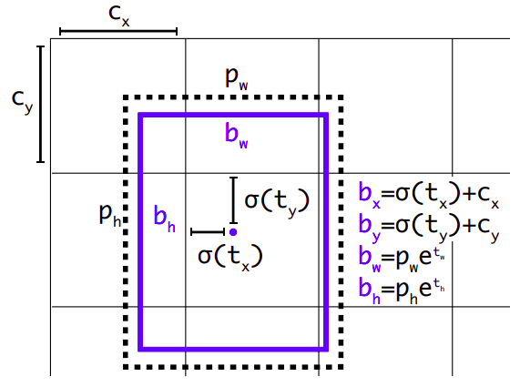
Predictions

for each cell and each anchor box the model will make a prediction that will contain:

• \(t_x\), \(t_y\): the offset of the object center to the cell’s top left corner.

• \(t_w\): \(t_y\): the widths of the object bounding box as referred to the anchor box size.

• \(t_0\): a proxy for the probability of an object’s center being present at that cell: \(Pr(object)*IOU(b, object)=\sigma(t_0)\)

• \(\mathbf{p}_c\): a vector of class probabilities

observe that:

• \(p_w\), \(p_h\) are the dimensions of the anchor box.

• the sigmoid function \(sigma\) is used to bound offset coordinates.

• the exponential function \(e\) is used to bound sizes \(>0\) and provide larger gradients when

• we are interested in both probability and IOU of the bounding box.

Therefore for each cell and anchor box we have \(5+C\) predictions, \(C\) being the number of classes in our dataset.

Image taken from YOLO9000: Better, Faster, Stronger

Image("local/imgs/yolo_predictions.png")

Typically, CNNs will

• downsample image dimensions to \(13x13\), or the number of cells defined, and will do a \((1,1)\) convolution in 2D with \(n_a(5+C)\) channels, \(n_a\) being the number of anchor boxes.

• make the same process in previous CNN layers (for instance when the activation map is \(52x52\)) or larger. So there is a set of prediction boxes

This will be ok to predict large object, but small ones get lost in CNN downsampling. To overcome this, different architectures use different techniques:

• YOLO3 make predictions in earlier CNN layers besides the last one.

• RetinaNet downsamples the image and then unsamples cativation maps, to integrate (sort of skipped connections) high level semantic information of late layers with spatial information from earlier layers.

See this blog for further intuitions on this

Loss function

Observe that we are doing BOTH regression (for boxes) AND classification (for object classes). A specific loss function must then be devised to take this into account.

See this blog post and this blog post for detailed explanations.

Non maximum suppression

Finally, as there might be many box predictions at different cells and resolutions, a decision must be taken for overlapping predictions. This is Non maximum suppression, and you can check this blog for a detailed explanation.