
3.4 - Batch normalization#
!wget -nc --no-cache -O init.py -q https://raw.githubusercontent.com/rramosp/2021.deeplearning/main/content/init.py
import init; init.init(force_download=False);
import numpy as np
import tensorflow as tf
import matplotlib.pyplot as plt
import pandas as pd
%matplotlib inline
%load_ext tensorboard

from sklearn.datasets import *
from local.lib import mlutils
tf.__version__
The tensorboard extension is already loaded. To reload it, use:
  %reload_ext tensorboard
'2.4.1'
Covariate shift#
Change of distribution of input to a function:
in input data it happens when using new data
in intermediate layers happens ALSO when previous layers change weights when training.
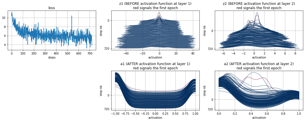
Covariate shift during training#
Observe how we use TF Low Level API and custom optimization to see the covariate shift during training
this could have been done also with the high level API and custom tensorboard summarizers
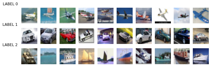
We are using again a small dataset based on CIFAR-10
!wget -nc https://s3.amazonaws.com/rlx/mini_cifar.h5
--2021-01-22 14:25:19--  https://s3.amazonaws.com/rlx/mini_cifar.h5
Resolving s3.amazonaws.com (s3.amazonaws.com)... 52.216.8.229
Connecting to s3.amazonaws.com (s3.amazonaws.com)|52.216.8.229|:443... connected.
HTTP request sent, awaiting response... 200 OK
Length: 14803609 (14M) [binary/octet-stream]
Saving to: ‘mini_cifar.h5’

mini_cifar.h5       100%[===================>]  14,12M  3,95MB/s    in 3,9s

2021-01-22 14:25:23 (3,58 MB/s) - ‘mini_cifar.h5’ saved [14803609/14803609]
import h5py
with h5py.File('mini_cifar.h5','r') as h5f:
    x_cifar = h5f["x"][:]
    y_cifar = h5f["y"][:]
mlutils.show_labeled_image_mosaic(x_cifar, y_cifar)
print(np.min(x_cifar), np.max(x_cifar))
0.0 1.0
from sklearn.model_selection import train_test_split
x_train, x_test, y_train, y_test = train_test_split(x_cifar, y_cifar, test_size=.25)
num_classes = len(np.unique(y_train))
print(x_train.shape, y_train.shape, x_test.shape, y_test.shape)
print("\ndistribution of train classes")
print(pd.Series(y_train).value_counts())
print("\ndistribution of test classes")
print(pd.Series(y_test).value_counts())
print("\nnum classes", num_classes)
x_train = x_train.astype(np.float32)
y_train = y_train.astype(np.float32)
x_test = x_test.astype(np.float32)
y_test = y_test.astype(np.float32)
(2253, 32, 32, 3) (2253,) (751, 32, 32, 3) (751,)

distribution of train classes
2    765
0    751
1    737
dtype: int64

distribution of test classes
2    260
0    254
1    237
dtype: int64

num classes 3
flatten data
x_trainf = np.r_[[i.flatten() for i in x_train]]
x_testf  = np.r_[[i.flatten() for i in x_test]]
x_trainf.shape, x_testf.shape
((2253, 3072), (751, 3072))
Set up a model with Keras and train#
from tensorflow.keras import Model
from tensorflow.keras.activations import relu, sigmoid, tanh, linear, softmax
from progressbar import progressbar as pbar
from scipy.stats import gaussian_kde

class MyModel(Model):

    def build(self, input_shape):

        self.w1 = self.add_weight(shape=(input_shape[-1], 100), initializer='random_normal', trainable=True, dtype=tf.float32)
        self.b1 = self.add_weight(shape=(100, ), initializer='random_normal', trainable=True, dtype=tf.float32)

        self.w2 = self.add_weight(shape=(100, 3), initializer='random_normal', trainable=True, dtype=tf.float32)
        self.b2 = self.add_weight(shape=(3, ), initializer='random_normal', trainable=True, dtype=tf.float32)

    @tf.function
    def get_z1(self, X):
        r = tf.matmul(X,self.w1)+self.b1
        return r

    @tf.function
    def get_a1(self, X):
        r = tf.tanh(self.get_z1(X))
        return r

    @tf.function
    def get_z2(self, X):
        a1 = self.get_a1(X)
        r = tf.matmul(a1,self.w2)+self.b2
        return r

    @tf.function
    def get_a2(self, X):
        return softmax(self.get_z2(X))

    @tf.function
    def call(self, X):
        a2 = self.get_a2(X)
        return a2

    @tf.function
    def train_step(self, X,y):
        preds = model(X)
        with tf.GradientTape() as tape:
            loss_value = tf.reduce_mean(self.loss(model(X), y))
        grads = tape.gradient(loss_value, self.trainable_variables)

        self.optimizer.apply_gradients(zip(grads, self.trainable_variables))
        return loss_value

    def fit(self, X,y, epochs=10, batch_size=32):
        self.hloss = []
        self.hz1, self.hz2 = [], []
        self.ha1, self.ha2 = [], []
        for epoch in pbar(range(epochs)):
            idxs = np.random.permutation(len(X))
            for step in range(len(X)//batch_size+((len(X)%batch_size)!=0)):

                X_batch = X[idxs][step*batch_size:(step+1)*batch_size]
                y_batch = y[idxs][step*batch_size:(step+1)*batch_size]
                loss_value = self.train_step(X_batch, y_batch)
                self.hz1.append(self.get_z1(X_batch).numpy().flatten())
                self.hz2.append(self.get_z2(X_batch).numpy().flatten())
                self.ha1.append(self.get_a1(X_batch).numpy().flatten())
                self.ha2.append(self.get_a2(X_batch).numpy().flatten())
                self.hloss.append(loss_value)

    def score(self, X, y):
        return np.mean(model.predict(X).argmax(axis=1) == y)

    def plot_hist(self):
        def plot_z_history(s):
            s = s[::5]
            for i,data in enumerate(pbar(s)):
                kde = gaussian_kde(data)
                xrange = np.linspace(np.min(data), np.max(data),100)
                plt.plot(xrange, kde(xrange)-i*.005,
                         color=plt.cm.RdBu(255*i/len(s)),
                         alpha=.5)
            plt.yticks([0,-i*.005], [0,len(model.hz1)]);
            plt.ylabel("step nb")
            plt.xlabel("activation")
            plt.grid();
        plt.figure(figsize=(15,6))
        plt.subplot(231)
        plt.plot(self.hloss); plt.grid(); plt.title("loss"); plt.xlabel("steps")
        plt.subplot(232)
        plot_z_history(self.hz1); plt.title("z1 (BEFORE activation function at layer 1)\nred signals the first epoch")
        plt.subplot(233)
        plot_z_history(self.hz2); plt.title("z2 (BEFORE activation function at layer 2)\nred signals the first epoch")
        plt.subplot(235)
        plot_z_history(self.ha1); plt.title("a1 (AFTER activation function at layer 1)\nred signals the first epoch")
        plt.subplot(236)
        plot_z_history(self.ha2); plt.title("a2 (AFTER activation function at layer 2)\nred signals the first epoch")
        plt.tight_layout()
from tensorflow.keras.optimizers import SGD, Adam
from tensorflow.keras.losses import categorical_crossentropy
model = MyModel()
model.compile(optimizer="adam", loss=categorical_crossentropy)
model.fit(x_trainf, np.eye(3)[y_train.astype(int)], epochs=20, batch_size=64)
print ("train accuracy %.3f"%model.score(x_trainf, y_train))
print ("test  accuracy %.3f"%model.score(x_testf, y_test))
model.plot_hist()
100% (20 of 20) |########################| Elapsed Time: 0:00:07 Time: 0:00:07
train accuracy 0.682
test  accuracy 0.593
100% (144 of 144) |######################| Elapsed Time: 0:00:01 Time:  0:00:01
100% (144 of 144) |######################| Elapsed Time: 0:00:00 Time:  0:00:00
100% (144 of 144) |######################| Elapsed Time: 0:00:01 Time:  0:00:01
100% (144 of 144) |######################| Elapsed Time: 0:00:00 Time:  0:00:00
Batch Normalizations fixes the covariate shift:
just before the linear network output is fed to the activation function
or just after
Recall the activation of any layer \(l\):
where \(a^{[l-1]}\) is the activation (output) of the previous layer, \(W^{[l]}\) and \(b^{[l]}\) are the layer weights, and \(\text{activation}\) is the activation function of that layer (relu, sigmoid, etc.). If layer \(l\) has \(n_l\) neurons, then \(z^{[l]}\) is a vector of \(n_l\) elements, just as \(b^{[l]}\) and \(a^{[l]}\)
if we normalize just before the activation function, we normalize \(z^{[l]}\) by substracting its mean and dividing by the standard deviation
so that:
where, \(\epsilon\) is a small number (such as 1e-3) for numerical stability in case the variace is very close to zero.
Scaling
Actually, we allow the normalization to have mean and std different from 0 and 1 respectively.
where \(\gamma^{[l]}\) and \(\beta^{[l]}\) are parameters learnable during training (with gradients, etc.)
Test data
When using test data, it might not have much sense to compute \(\mu\) and \(\sigma\) for small batches (at the extreme the batch size could even be 1, to obtain a prediction for a single data point). In these cases, a running averate of both \(\mu\) and \(\sigma\) are kept during training and the used in test.
Other issues
BN can be seen as a mild form of regularization, since using \(\mu\) and \(\sigma\) for every batch introduces some noise during training (such as dropout)
\(\beta^{[l]}\) will subsume the bias parameter of the layer, as they end up being scaled and summed without depending on the data. They both act as constants which can be integrated in a single constant parameter.
See