4.1 - Convolutions

!wget -nc --no-cache -O init.py -q https://raw.githubusercontent.com/rramosp/2021.deeplearning/main/content/init.py
import init; init.init(force_download=False); 

import numpy as np
import tensorflow as tf
import matplotlib.pyplot as plt
from skimage.io import imread
from scipy import signal
%matplotlib inline
tf.__version__

'2.4.1'

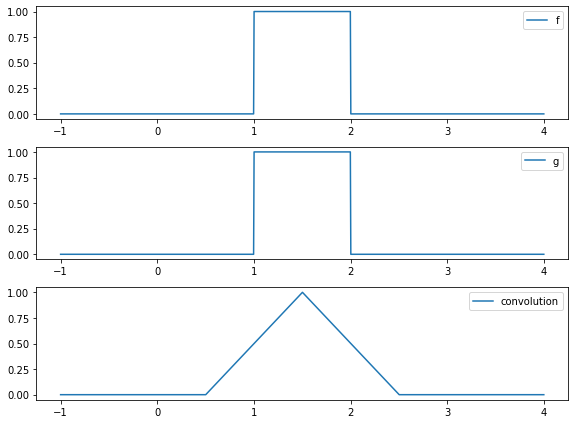
Convolutions of functions

A convolution is a mathematical operations that receives as input two functions and produces as output another function.

The intuition is that one input function sweeps over the second input function and they get multiplied along the way.

See Wikipedia:Convolution

\[(f*g)(t) = \int_{-\infty}^\infty f(t)g(t-\tau)d\tau\]

f = lambda x: ((x>1) & (x<2)).astype(int)
g = lambda x: ((x>1) & (x<2)).astype(int)

x = np.linspace(-1,4,1000)
c = np.convolve(f(x),g(x), "same")
c = c/np.max(c)

plt.figure(figsize=(8,6))
plt.subplot(311); plt.plot(x,f(x), label="f"); plt.legend()
plt.subplot(312); plt.plot(x,g(x), label="g"); plt.legend()
plt.subplot(313); plt.plot(x,c, label="convolution"); plt.legend()
plt.tight_layout()

Convolution is just multiplication and adding

In a discrete setting, integration becomes summation.

\[(f*g)[t] = \sum_{i=-\infty}^{+\infty} f[t]g[t-i]\]

a = np.r_[0,0,1,1,1,0,0]
b = np.r_[0,0,1,1,1,0,0]
np.convolve(a,b)

array([0, 0, 0, 0, 1, 2, 3, 2, 1, 0, 0, 0, 0])

observe each convolution step is just an element by element multiplication of vectors and a sumation of the resulting elements.

for i in range(len(a)*2-1):
    pa, pb = (a[:i+1], b[-i-1:]) if i < len(a) else (a[i-len(a)+1:], b[:-(i-len(a))-1])
    print ((pa*pb).sum(), "=", pa, "*", pb)

0 = [0] * [0]
0 = [0 0] * [0 0]
0 = [0 0 1] * [1 0 0]
0 = [0 0 1 1] * [1 1 0 0]
1 = [0 0 1 1 1] * [1 1 1 0 0]
2 = [0 0 1 1 1 0] * [0 1 1 1 0 0]
3 = [0 0 1 1 1 0 0] * [0 0 1 1 1 0 0]
2 = [0 1 1 1 0 0] * [0 0 1 1 1 0]
1 = [1 1 1 0 0] * [0 0 1 1 1]
0 = [1 1 0 0] * [0 0 1 1]
0 = [1 0 0] * [0 0 1]
0 = [0 0] * [0 0]
0 = [0] * [0]

the mode argument to convolve regulates padding

np.convolve(a,b, mode="same")

array([0, 1, 2, 3, 2, 1, 0])

Of course, the functions can have any values, and not necessarily be the same, and we assume there is infinity zero padding on both arguments, so they do not have to be the same size.

In this case:

• a is considered the source signal

• b is considered the filter

a = np.r_[0,0,1,1,1,0,0]
b = np.r_[1,0,1]
np.convolve(a,b)

array([0, 0, 1, 1, 2, 1, 1, 0, 0])

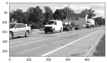
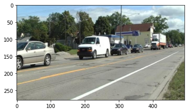
Convolution with images

It is simply sweeping in both directions

img = imread("local/imgs/cars-driving.jpg").mean(axis=2)
img = (img-np.min(img))/(np.max(img)-np.min(img)) # normalize to 0,1
img.shape, np.min(img), np.max(img)

((278, 493), 0.0, 1.0)

plt.imshow(img, cmap=plt.cm.Greys_r)

<matplotlib.image.AxesImage at 0x7fb9302c3a30>

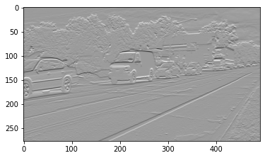
a conv 2D is just the same element by element multiplication and summation.

f1 = np.r_[[[-1,-1], [1,1]]]
print (f1)
c1 = signal.convolve2d(img, f1, mode="valid")

[[-1 -1]
 [ 1  1]]

doing manually the first pixel of the resulting img

c1[0,1], (img[:2,:2]*f1).sum()

(0.002645502645502562, -0.002645502645502562)

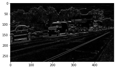
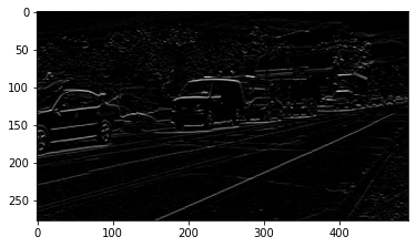
and this filter has a border detection effect.

plt.imshow(c1, cmap=plt.cm.Greys_r)

<matplotlib.image.AxesImage at 0x7fb948229b80>

We use abs con convert all differences into positive, since we do not care the direction of edges.

plt.imshow(np.abs(c1), cmap=plt.cm.Greys_r)

<matplotlib.image.AxesImage at 0x7fb948568190>

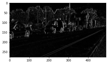
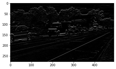
and a filter for vertical edge detection

f2 = np.r_[[[1,-1], [1,-1]]]
print(f)
c2 = signal.convolve2d(img, f2, mode="valid")
plt.imshow(np.abs(c2), cmap=plt.cm.Greys_r)

[[ 1 -1]
 [ 1 -1]]

<matplotlib.image.AxesImage at 0x7fb948308430>

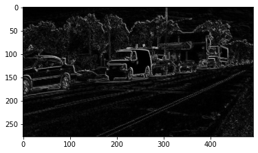
combining both outputs

plt.imshow(np.abs(c1+c2), cmap=plt.cm.Greys_r)

<matplotlib.image.AxesImage at 0x7fb949422130>

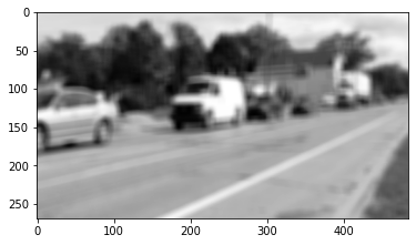
a blurring filter

f = np.ones((10,10))
print(f)
c = signal.convolve2d(img, f, mode="valid")
plt.imshow(np.abs(c), cmap=plt.cm.Greys_r)

[[1. 1. 1. 1. 1. 1. 1. 1. 1. 1.]
 [1. 1. 1. 1. 1. 1. 1. 1. 1. 1.]
 [1. 1. 1. 1. 1. 1. 1. 1. 1. 1.]
 [1. 1. 1. 1. 1. 1. 1. 1. 1. 1.]
 [1. 1. 1. 1. 1. 1. 1. 1. 1. 1.]
 [1. 1. 1. 1. 1. 1. 1. 1. 1. 1.]
 [1. 1. 1. 1. 1. 1. 1. 1. 1. 1.]
 [1. 1. 1. 1. 1. 1. 1. 1. 1. 1.]
 [1. 1. 1. 1. 1. 1. 1. 1. 1. 1.]
 [1. 1. 1. 1. 1. 1. 1. 1. 1. 1.]]

<matplotlib.image.AxesImage at 0x7f1e015a4250>

In Tensorflow in just the same

TF usually expects an array of imgs of shape

(n_imgs, pixels_width, pixels_height, n_channels)

# reshape image
img = imread("local/imgs/cars-driving.jpg").mean(axis=2)
img = (img-np.min(img))/(np.max(img)-np.min(img)) # normalize to 0,1
img = img.reshape(1,*img.shape,1)
img.shape

(1, 278, 493, 1)

we want one filter of size 2x2

c = tf.keras.layers.Conv2D(filters=1, kernel_size=2, activation="linear", padding="same")
c.build(input_shape=(img.shape))

for w in c.weights:
    print (w)

<tf.Variable 'kernel:0' shape=(2, 2, 1, 1) dtype=float32, numpy=
array([[[[-0.45081097]],

        [[ 0.6782841 ]]],


       [[[ 0.31860155]],

        [[-0.4256522 ]]]], dtype=float32)>
<tf.Variable 'bias:0' shape=(1,) dtype=float32, numpy=array([0.], dtype=float32)>

manually set the filter values

c.set_weights([ np.r_[[[-1,-1], [1,1]]].reshape(2,2,1,1), np.r_[0]])

cimg = c(img)
cimg.shape

TensorShape([1, 278, 493, 1])

cimg[0,0,0]

<tf.Tensor: shape=(1,), dtype=float32, numpy=array([-0.00264549], dtype=float32)>

plt.imshow(np.abs(cimg.numpy()[0,:,:,0]), cmap=plt.cm.Greys_r)

<matplotlib.image.AxesImage at 0x7fb930373be0>

cimg[0,0,0]

<tf.Tensor: shape=(1,), dtype=float32, numpy=array([-0.00264549], dtype=float32)>

(img[0,:2,:2,0]*np.r_[[[-1,-1], [1,1]]]).sum()

-0.002645502645502562

activations are simply applied to the output. Observe how a relu activation with an horizontal edge detection filter detects edges in one direction

c = tf.keras.layers.Conv2D(filters=1, kernel_size=2, activation="relu", padding="valid")
c.build(input_shape=(img.shape))
c.set_weights([ np.r_[[[-1,-1], [1,1]]].reshape(2,2,1,1), np.r_[0]])
plt.imshow(c(img).numpy()[0,:,:,0], cmap=plt.cm.Greys_r)

<matplotlib.image.AxesImage at 0x7fb930518160>

or the other direcction inverting the filter

c = tf.keras.layers.Conv2D(filters=1, kernel_size=2, activation="relu", padding="valid")
c.build(input_shape=(img.shape))
c.set_weights([ np.r_[[[1,1], [-1,-1]]].reshape(2,2,1,1), np.r_[0]])
plt.imshow(c(img).numpy()[0,:,:,0], cmap=plt.cm.Greys_r)

<matplotlib.image.AxesImage at 0x7fb9304e6280>

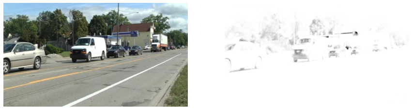
for color images, filters also have to have three channels

img = imread("local/imgs/cars-driving.jpg")
img = (img-np.min(img))/(np.max(img)-np.min(img)) # normalize to 0,1
img = img.reshape(1, *img.shape)
plt.imshow(img[0])

<matplotlib.image.AxesImage at 0x7fb9304afa30>

f = -np.ones((3,3,3))*1.5
f[:,:,0] = 1.5
f

array([[[ 1.5, -1.5, -1.5],
        [ 1.5, -1.5, -1.5],
        [ 1.5, -1.5, -1.5]],

       [[ 1.5, -1.5, -1.5],
        [ 1.5, -1.5, -1.5],
        [ 1.5, -1.5, -1.5]],

       [[ 1.5, -1.5, -1.5],
        [ 1.5, -1.5, -1.5],
        [ 1.5, -1.5, -1.5]]])

c = tf.keras.layers.Conv2D(filters=1, kernel_size=3, activation="sigmoid", padding="valid")
c.build(input_shape=(img.shape))
c.set_weights([ f.reshape(3,3,3,1), np.r_[0]])

cimg = c(img).numpy()
cimg.shape

(1, 276, 491, 1)

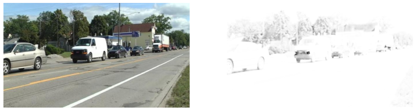
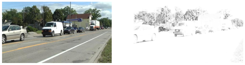
observe how very pure red is detected (hand crafted filter is difficult to tune)

plt.figure(figsize=(15,10))
plt.subplot(121); plt.imshow(img[0,:,:]); plt.axis("off")
plt.subplot(122); plt.imshow(cimg[0,:,:,0], cmap=plt.cm.Greys); plt.axis("off")

(-0.5, 490.5, 275.5, -0.5)

detect green (little)

f = -np.ones((3,3,3))*1.5
f[:,:,1] = 1.5
c.set_weights([ f.reshape(3,3,3,1), np.r_[0]])
plt.figure(figsize=(15,10))
cimg = c(img).numpy()

plt.subplot(121); plt.imshow(img[0,:,:]); plt.axis("off")
plt.subplot(122); plt.imshow(cimg[0,:,:,0], cmap=plt.cm.Greys); plt.axis("off")

(-0.5, 490.5, 275.5, -0.5)

detect blue (little tolerace)

f = -np.ones((3,3,3))*1.5
f[:,:,2] = 1.5
c.set_weights([ f.reshape(3,3,3,1), np.r_[0]])
plt.figure(figsize=(15,10))
cimg = c(img).numpy()

plt.subplot(121); plt.imshow(img[0,:,:]); plt.axis("off")
plt.subplot(122); plt.imshow(cimg[0,:,:,0], cmap=plt.cm.Greys); plt.axis("off")

(-0.5, 490.5, 275.5, -0.5)