
4.2 - Convolutional Neural Networks#
Course’s material requires a tensorflow version lower than the default one used in Google Colab. Run the following cell to downgrade TensorFlow accordingly.
!wget -nc --no-cache -O init.py -q https://raw.githubusercontent.com/rramosp/2021.deeplearning/main/content/init.py
import init; init.init(force_download=False);
/content/init.py:2: SyntaxWarning: invalid escape sequence '\S'
  course_id = '\S*deeplearning\S*'
replicating local resources
import tensorflow as tf
from time import time
import pandas as pd
import matplotlib.pyplot as plt
import numpy as np
from local.lib import mlutils
%matplotlib inline
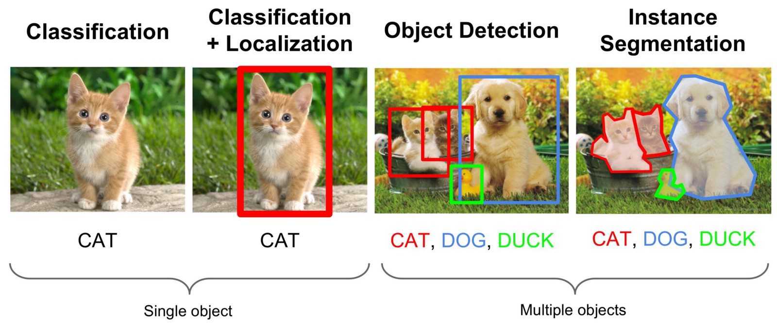
Image analytics tasks#
from IPython.display import Image
Image(filename='local/imgs/imgs_tasks.jpeg', width=800)
Explore COCO Dataset#
also
Image APIs Clarifai Amazon Rekognition, Google Cloud Vision
Image Captioning (con CNN + RNN!!!) caption bot
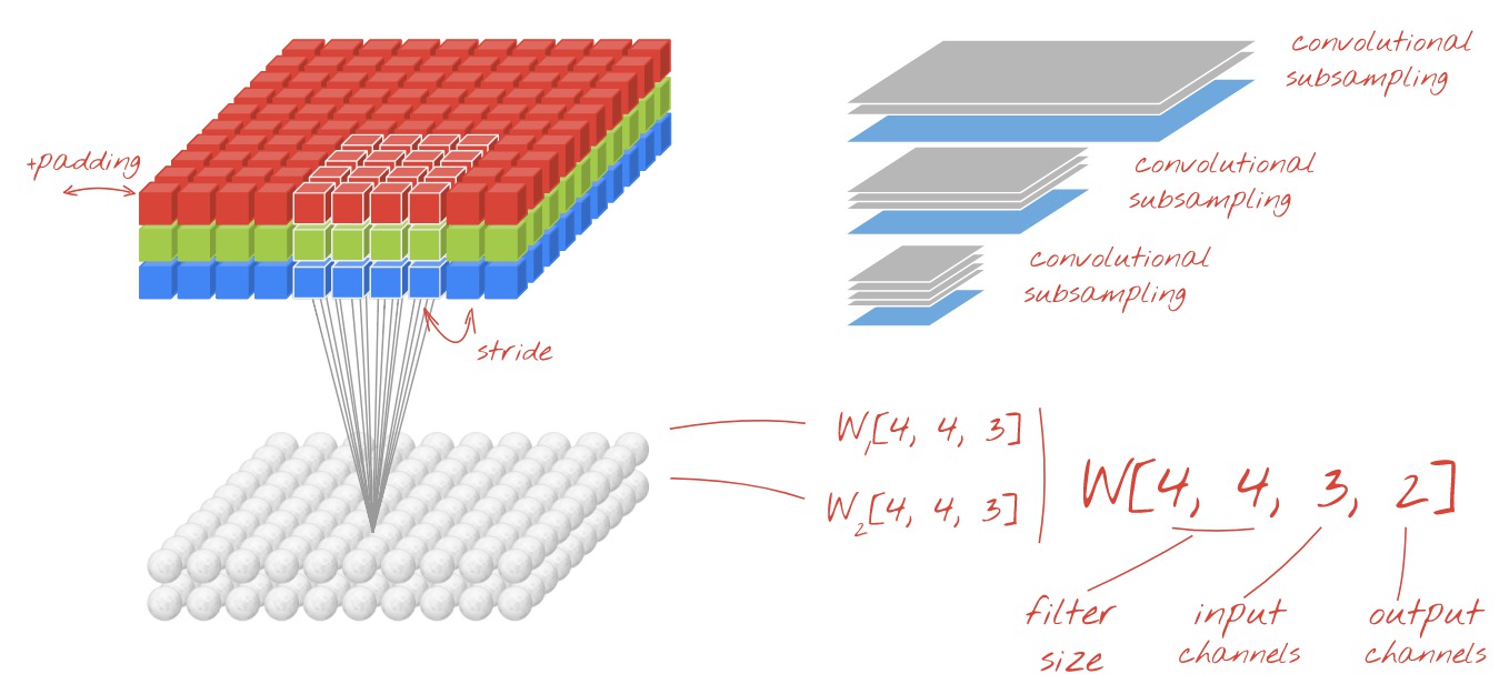
Convolutional Neural Networks#
see video series Tensorflow and Deep Learning without a PhD
see convolutions summary | filter activation demo | confusion matrix
see The 9 Deep Learning Papers You Should Know
RECOMMENDATION#
close all applications
install Maxthon browser http://www.maxthon.com
open only VirtualBox and Maxthon
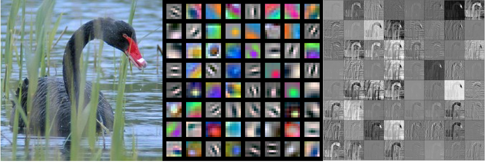
First level filters and activations maps#
the filters in the middle are applied to the image on the left. Observe, for instance, in what parts of the image the seventh filter of the first row is activated (the one before the last one in the first row).
Image(filename='local/imgs/cnn_swan.png', width=800)
Hierarchy of filters and activation maps#
Image(filename='local/imgs/cnn_features.png', width=600)
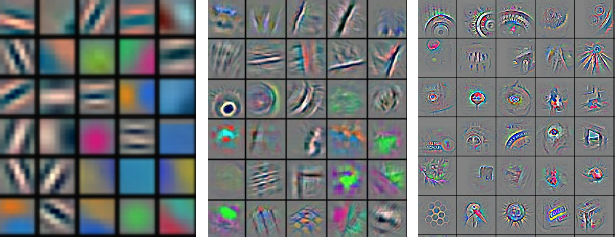
Image(filename='local/imgs/conv1.jpg', width=800)
Image(filename='local/imgs/conv2.jpg', width=800)
otros ejemplos de filtros de primer nivel
Image(filename='local/imgs/cnn_features2.png', width=600)
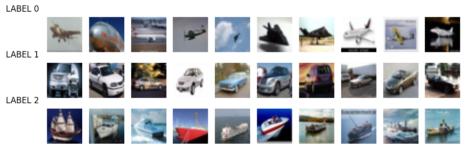
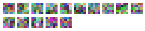
We have a small image dataset based on CIFAR-10, where each image size is 32x32x3.
!wget -nc https://s3.amazonaws.com/rlx/mini_cifar.h5
--2025-09-03 22:13:45--  https://s3.amazonaws.com/rlx/mini_cifar.h5
Resolving s3.amazonaws.com (s3.amazonaws.com)... 3.5.21.44, 52.217.172.48, 3.5.24.43, ...
Connecting to s3.amazonaws.com (s3.amazonaws.com)|3.5.21.44|:443... connected.
HTTP request sent, awaiting response... 200 OK
Length: 14803609 (14M) [binary/octet-stream]
Saving to: ‘mini_cifar.h5’

mini_cifar.h5       100%[===================>]  14.12M  66.7MB/s    in 0.2s

2025-09-03 22:13:45 (66.7 MB/s) - ‘mini_cifar.h5’ saved [14803609/14803609]
import h5py
with h5py.File('mini_cifar.h5','r') as h5f:
    x_cifar = h5f["x"][:]
    y_cifar = h5f["y"][:]
mlutils.show_labeled_image_mosaic(x_cifar, y_cifar)
print (np.min(x_cifar), np.max(x_cifar))
0.0 1.0
from sklearn.model_selection import train_test_split
x_train, x_test, y_train, y_test = train_test_split(x_cifar, y_cifar, test_size=.25)
print (x_train.shape, y_train.shape, x_test.shape, y_test.shape)
print ("\ndistribution of train classes")
print (pd.Series(y_train).value_counts())
print ("\ndistribution of test classes")
print (pd.Series(y_test).value_counts())
(2253, 32, 32, 3) (2253,) (751, 32, 32, 3) (751,)

distribution of train classes
2    788
0    750
1    715
Name: count, dtype: int64

distribution of test classes
1    259
0    255
2    237
Name: count, dtype: int64
build a Keras model
def get_conv_model_A(num_classes, img_size=32, compile=True):
    tf.keras.backend.clear_session()
    print ("using",num_classes,"classes")
    inputs = tf.keras.Input(shape=(img_size,img_size,3), name="input_1")
    layers = tf.keras.layers.Conv2D(15,(3,3), activation="relu", padding="SAME")(inputs)
    layers = tf.keras.layers.Flatten()(layers)
    layers = tf.keras.layers.Dense(16, activation=tf.nn.relu)(layers)
    layers = tf.keras.layers.Dropout(0.2)(layers)
    predictions = tf.keras.layers.Dense(num_classes, activation=tf.nn.softmax, name="output_1")(layers)
    model = tf.keras.Model(inputs = inputs, outputs=predictions)
    if compile:
        model.compile(optimizer='adam',
                      loss='sparse_categorical_crossentropy',
                      metrics=['accuracy'])
    return model
num_classes = len(np.unique(y_cifar))
model = get_conv_model_A(num_classes)
using 3 classes
observe the weights initialized and their weights
weights = model.get_weights()
for i in weights:
    print (i.shape)
(3, 3, 3, 15)
(15,)
(15360, 16)
(16,)
(16, 3)
(3,)
we keep the filters on the first layer to later compare them with the same filters after training.
initial_w0 = model.get_weights()[0].copy()
y_test.shape, y_train.shape, x_test.shape, x_train.shape
((751,), (2253,), (751, 32, 32, 3), (2253, 32, 32, 3))
num_classes = len(np.unique(y_cifar))

def train(model, batch_size, epochs, model_name=""):
    tensorboard = tf.keras.callbacks.TensorBoard(log_dir="logs/"+model_name+"_"+"{}".format(time()))
    model.fit(x_train, y_train, epochs=epochs, callbacks=[tensorboard],
              batch_size=batch_size,
              validation_data=(x_test, y_test))
    metrics = model.evaluate(x_test, y_test)
    return {k:v for k,v in zip (model.metrics_names, metrics)}
observe the shapes of model weights obtained above and try to see how they are related to the output shape and the number of parameters
model = get_conv_model_A(num_classes)
model.summary()
using 3 classes
Model: "functional"
┏━━━━━━━━━━━━━━━━━━━━━━━━━━━━━━━━━┳━━━━━━━━━━━━━━━━━━━━━━━━┳━━━━━━━━━━━━━━━┓
┃ Layer (type)                    ┃ Output Shape           ┃       Param # ┃
┡━━━━━━━━━━━━━━━━━━━━━━━━━━━━━━━━━╇━━━━━━━━━━━━━━━━━━━━━━━━╇━━━━━━━━━━━━━━━┩
│ input_1 (InputLayer)            │ (None, 32, 32, 3)      │             0 │
├─────────────────────────────────┼────────────────────────┼───────────────┤
│ conv2d (Conv2D)                 │ (None, 32, 32, 15)     │           420 │
├─────────────────────────────────┼────────────────────────┼───────────────┤
│ flatten (Flatten)               │ (None, 15360)          │             0 │
├─────────────────────────────────┼────────────────────────┼───────────────┤
│ dense (Dense)                   │ (None, 16)             │       245,776 │
├─────────────────────────────────┼────────────────────────┼───────────────┤
│ dropout (Dropout)               │ (None, 16)             │             0 │
├─────────────────────────────────┼────────────────────────┼───────────────┤
│ output_1 (Dense)                │ (None, 3)              │            51 │
└─────────────────────────────────┴────────────────────────┴───────────────┘
Total params: 246,247 (961.90 KB)
Trainable params: 246,247 (961.90 KB)
Non-trainable params: 0 (0.00 B)
train(model, batch_size=32, epochs=10, model_name="model_A")
Epoch 1/10
71/71 ━━━━━━━━━━━━━━━━━━━━ 4s 33ms/step - accuracy: 0.4473 - loss: 1.2124 - val_accuracy: 0.6405 - val_loss: 0.8304
Epoch 2/10
71/71 ━━━━━━━━━━━━━━━━━━━━ 1s 19ms/step - accuracy: 0.6213 - loss: 0.8343 - val_accuracy: 0.6578 - val_loss: 0.7908
Epoch 3/10
71/71 ━━━━━━━━━━━━━━━━━━━━ 3s 19ms/step - accuracy: 0.6574 - loss: 0.7616 - val_accuracy: 0.6897 - val_loss: 0.7229
Epoch 4/10
71/71 ━━━━━━━━━━━━━━━━━━━━ 1s 17ms/step - accuracy: 0.6527 - loss: 0.7387 - val_accuracy: 0.7031 - val_loss: 0.7145
Epoch 5/10
71/71 ━━━━━━━━━━━━━━━━━━━━ 1s 17ms/step - accuracy: 0.6950 - loss: 0.6999 - val_accuracy: 0.6937 - val_loss: 0.7106
Epoch 6/10
71/71 ━━━━━━━━━━━━━━━━━━━━ 1s 17ms/step - accuracy: 0.7206 - loss: 0.6592 - val_accuracy: 0.6897 - val_loss: 0.7089
Epoch 7/10
71/71 ━━━━━━━━━━━━━━━━━━━━ 1s 17ms/step - accuracy: 0.7170 - loss: 0.6470 - val_accuracy: 0.7044 - val_loss: 0.6813
Epoch 8/10
71/71 ━━━━━━━━━━━━━━━━━━━━ 1s 19ms/step - accuracy: 0.7434 - loss: 0.5900 - val_accuracy: 0.7044 - val_loss: 0.6998
Epoch 9/10
71/71 ━━━━━━━━━━━━━━━━━━━━ 3s 21ms/step - accuracy: 0.7374 - loss: 0.5816 - val_accuracy: 0.7403 - val_loss: 0.6335
Epoch 10/10
71/71 ━━━━━━━━━━━━━━━━━━━━ 1s 19ms/step - accuracy: 0.7540 - loss: 0.5684 - val_accuracy: 0.7350 - val_loss: 0.6252
24/24 ━━━━━━━━━━━━━━━━━━━━ 0s 7ms/step - accuracy: 0.7377 - loss: 0.6379
{'loss': 0.6252090930938721, 'compile_metrics': 0.7350199818611145}
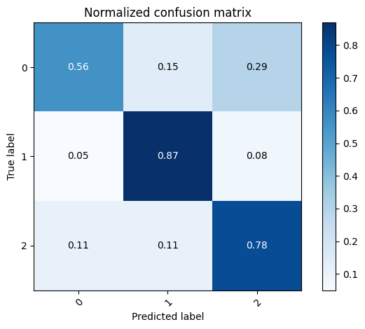
test_preds = model.predict(x_test).argmax(axis=1)
mlutils.plot_confusion_matrix(y_test, test_preds, classes=np.r_[0,1,2], normalize=True)
24/24 ━━━━━━━━━━━━━━━━━━━━ 0s 7ms/step
Normalized confusion matrix
[[0.56078431 0.14509804 0.29411765]
 [0.05019305 0.86872587 0.08108108]
 [0.11392405 0.10970464 0.77637131]]
<Axes: title={'center': 'Normalized confusion matrix'}, xlabel='Predicted label', ylabel='True label'>
observe the outp in tensorboard
tensorboard --logdir logs
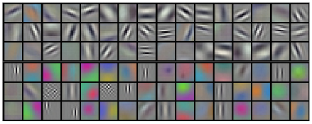
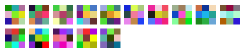
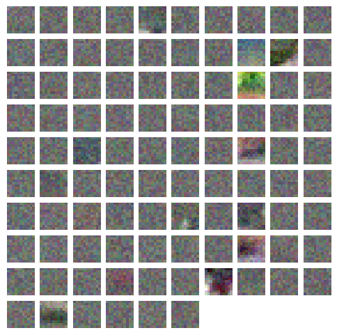
first layer filters before training
mlutils.display_imgs(initial_w0)
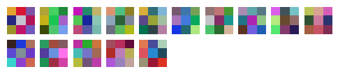
and after training
w0 = model.get_weights()[0]
print (w0.shape)
mlutils.display_imgs(w0)
(3, 3, 3, 15)
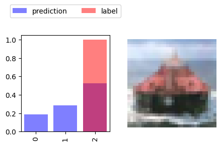
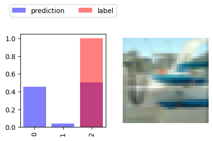
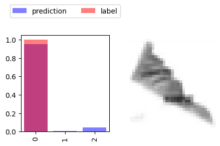
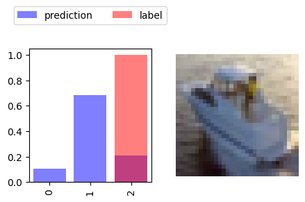
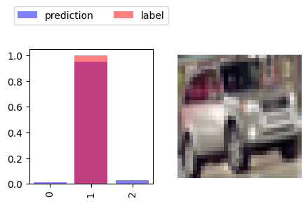
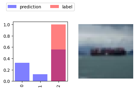
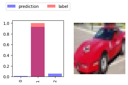
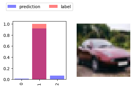
idxs = np.random.permutation(len(x_test))[:5]
preds = model.predict(x_test[idxs])
mlutils.show_preds(x_test[idxs],y_test[idxs], preds)
1/1 ━━━━━━━━━━━━━━━━━━━━ 0s 53ms/step
Let’s try a more complex network#
def get_conv_model_B(num_classes, img_size=32, compile=True):
    tf.keras.backend.clear_session()
    print ("using",num_classes,"classes")
    inputs = tf.keras.Input(shape=(img_size,img_size,3), name="input_1")
    layers = tf.keras.layers.Conv2D(15,(5,5), activation="relu")(inputs)
    layers = tf.keras.layers.MaxPool2D((2,2))(layers)
    layers = tf.keras.layers.Conv2D(60,(5,5), activation="relu")(layers)
    layers = tf.keras.layers.Flatten()(layers)
    layers = tf.keras.layers.Dense(16, activation=tf.nn.relu)(layers)
    layers = tf.keras.layers.Dropout(0.2)(layers)
    predictions = tf.keras.layers.Dense(num_classes, activation=tf.nn.softmax, name="output_1")(layers)
    model = tf.keras.Model(inputs = inputs, outputs=predictions)
    if compile:
        model.compile(optimizer='adam',
                      loss='sparse_categorical_crossentropy',
                      metrics=['accuracy'])
    return model
model = get_conv_model_B(num_classes)
model.summary()
train(model, batch_size=32, epochs=10, model_name="model_B")
using 3 classes
Model: "functional"
┏━━━━━━━━━━━━━━━━━━━━━━━━━━━━━━━━━┳━━━━━━━━━━━━━━━━━━━━━━━━┳━━━━━━━━━━━━━━━┓
┃ Layer (type)                    ┃ Output Shape           ┃       Param # ┃
┡━━━━━━━━━━━━━━━━━━━━━━━━━━━━━━━━━╇━━━━━━━━━━━━━━━━━━━━━━━━╇━━━━━━━━━━━━━━━┩
│ input_1 (InputLayer)            │ (None, 32, 32, 3)      │             0 │
├─────────────────────────────────┼────────────────────────┼───────────────┤
│ conv2d (Conv2D)                 │ (None, 28, 28, 15)     │         1,140 │
├─────────────────────────────────┼────────────────────────┼───────────────┤
│ max_pooling2d (MaxPooling2D)    │ (None, 14, 14, 15)     │             0 │
├─────────────────────────────────┼────────────────────────┼───────────────┤
│ conv2d_1 (Conv2D)               │ (None, 10, 10, 60)     │        22,560 │
├─────────────────────────────────┼────────────────────────┼───────────────┤
│ flatten (Flatten)               │ (None, 6000)           │             0 │
├─────────────────────────────────┼────────────────────────┼───────────────┤
│ dense (Dense)                   │ (None, 16)             │        96,016 │
├─────────────────────────────────┼────────────────────────┼───────────────┤
│ dropout (Dropout)               │ (None, 16)             │             0 │
├─────────────────────────────────┼────────────────────────┼───────────────┤
│ output_1 (Dense)                │ (None, 3)              │            51 │
└─────────────────────────────────┴────────────────────────┴───────────────┘
Total params: 119,767 (467.84 KB)
Trainable params: 119,767 (467.84 KB)
Non-trainable params: 0 (0.00 B)
Epoch 1/10
71/71 ━━━━━━━━━━━━━━━━━━━━ 4s 37ms/step - accuracy: 0.4160 - loss: 1.0678 - val_accuracy: 0.5885 - val_loss: 0.9273
Epoch 2/10
71/71 ━━━━━━━━━━━━━━━━━━━━ 4s 52ms/step - accuracy: 0.5649 - loss: 0.9118 - val_accuracy: 0.6125 - val_loss: 0.8346
Epoch 3/10
71/71 ━━━━━━━━━━━━━━━━━━━━ 4s 34ms/step - accuracy: 0.5947 - loss: 0.8255 - val_accuracy: 0.6911 - val_loss: 0.7538
Epoch 4/10
71/71 ━━━━━━━━━━━━━━━━━━━━ 2s 34ms/step - accuracy: 0.6596 - loss: 0.7524 - val_accuracy: 0.6937 - val_loss: 0.7103
Epoch 5/10
71/71 ━━━━━━━━━━━━━━━━━━━━ 3s 34ms/step - accuracy: 0.6510 - loss: 0.7328 - val_accuracy: 0.7137 - val_loss: 0.6942
Epoch 6/10
71/71 ━━━━━━━━━━━━━━━━━━━━ 4s 53ms/step - accuracy: 0.6763 - loss: 0.7173 - val_accuracy: 0.7217 - val_loss: 0.6599
Epoch 7/10
71/71 ━━━━━━━━━━━━━━━━━━━━ 4s 35ms/step - accuracy: 0.7023 - loss: 0.6559 - val_accuracy: 0.7417 - val_loss: 0.6539
Epoch 8/10
71/71 ━━━━━━━━━━━━━━━━━━━━ 2s 34ms/step - accuracy: 0.7208 - loss: 0.6330 - val_accuracy: 0.7590 - val_loss: 0.6169
Epoch 9/10
71/71 ━━━━━━━━━━━━━━━━━━━━ 3s 35ms/step - accuracy: 0.7530 - loss: 0.5603 - val_accuracy: 0.7590 - val_loss: 0.5748
Epoch 10/10
71/71 ━━━━━━━━━━━━━━━━━━━━ 4s 53ms/step - accuracy: 0.7677 - loss: 0.5238 - val_accuracy: 0.7523 - val_loss: 0.6104
24/24 ━━━━━━━━━━━━━━━━━━━━ 0s 12ms/step - accuracy: 0.7349 - loss: 0.6249
{'loss': 0.6103829145431519, 'compile_metrics': 0.7523302435874939}
w0 = model.get_weights()[0]
print (w0.shape)
mlutils.display_imgs(w0)
(5, 5, 3, 15)
or with larger filters#
def get_conv_model_C(num_classes, img_size=32, compile=True):
    tf.keras.backend.clear_session()
    print ("using",num_classes,"classes")
    inputs = tf.keras.Input(shape=(img_size,img_size,3), name="input_1")
    layers = tf.keras.layers.Conv2D(96,(11,11), activation="relu")(inputs)
    layers = tf.keras.layers.MaxPool2D((2,2))(layers)
    layers = tf.keras.layers.Conv2D(60,(11,11), activation="relu")(layers)
    layers = tf.keras.layers.Flatten()(layers)
    layers = tf.keras.layers.Dense(16, activation=tf.nn.relu)(layers)
    layers = tf.keras.layers.Dropout(0.2)(layers)
    predictions = tf.keras.layers.Dense(num_classes, activation=tf.nn.softmax, name="output_1")(layers)
    model = tf.keras.Model(inputs = inputs, outputs=predictions)
    if compile:
        model.compile(optimizer='adam',
                      loss='sparse_categorical_crossentropy',
                      metrics=['accuracy'])
    return model
model = get_conv_model_C(num_classes)
model.summary()
train(model, batch_size=32, epochs=10, model_name="model_C")
using 3 classes
Model: "functional"
┏━━━━━━━━━━━━━━━━━━━━━━━━━━━━━━━━━┳━━━━━━━━━━━━━━━━━━━━━━━━┳━━━━━━━━━━━━━━━┓
┃ Layer (type)                    ┃ Output Shape           ┃       Param # ┃
┡━━━━━━━━━━━━━━━━━━━━━━━━━━━━━━━━━╇━━━━━━━━━━━━━━━━━━━━━━━━╇━━━━━━━━━━━━━━━┩
│ input_1 (InputLayer)            │ (None, 32, 32, 3)      │             0 │
├─────────────────────────────────┼────────────────────────┼───────────────┤
│ conv2d (Conv2D)                 │ (None, 22, 22, 96)     │        34,944 │
├─────────────────────────────────┼────────────────────────┼───────────────┤
│ max_pooling2d (MaxPooling2D)    │ (None, 11, 11, 96)     │             0 │
├─────────────────────────────────┼────────────────────────┼───────────────┤
│ conv2d_1 (Conv2D)               │ (None, 1, 1, 60)       │       697,020 │
├─────────────────────────────────┼────────────────────────┼───────────────┤
│ flatten (Flatten)               │ (None, 60)             │             0 │
├─────────────────────────────────┼────────────────────────┼───────────────┤
│ dense (Dense)                   │ (None, 16)             │           976 │
├─────────────────────────────────┼────────────────────────┼───────────────┤
│ dropout (Dropout)               │ (None, 16)             │             0 │
├─────────────────────────────────┼────────────────────────┼───────────────┤
│ output_1 (Dense)                │ (None, 3)              │            51 │
└─────────────────────────────────┴────────────────────────┴───────────────┘
Total params: 732,991 (2.80 MB)
Trainable params: 732,991 (2.80 MB)
Non-trainable params: 0 (0.00 B)
Epoch 1/10
71/71 ━━━━━━━━━━━━━━━━━━━━ 8s 99ms/step - accuracy: 0.3655 - loss: 1.1214 - val_accuracy: 0.5140 - val_loss: 0.9933
Epoch 2/10
71/71 ━━━━━━━━━━━━━━━━━━━━ 8s 114ms/step - accuracy: 0.5219 - loss: 0.9886 - val_accuracy: 0.5965 - val_loss: 0.8874
Epoch 3/10
71/71 ━━━━━━━━━━━━━━━━━━━━ 10s 115ms/step - accuracy: 0.5585 - loss: 0.9041 - val_accuracy: 0.6138 - val_loss: 0.8526
Epoch 4/10
71/71 ━━━━━━━━━━━━━━━━━━━━ 11s 120ms/step - accuracy: 0.5946 - loss: 0.8621 - val_accuracy: 0.6431 - val_loss: 0.8478
Epoch 5/10
71/71 ━━━━━━━━━━━━━━━━━━━━ 7s 97ms/step - accuracy: 0.5931 - loss: 0.8814 - val_accuracy: 0.6471 - val_loss: 0.8161
Epoch 6/10
71/71 ━━━━━━━━━━━━━━━━━━━━ 11s 110ms/step - accuracy: 0.6173 - loss: 0.8420 - val_accuracy: 0.6471 - val_loss: 0.8194
Epoch 7/10
71/71 ━━━━━━━━━━━━━━━━━━━━ 11s 115ms/step - accuracy: 0.6380 - loss: 0.8193 - val_accuracy: 0.6485 - val_loss: 0.8030
Epoch 8/10
71/71 ━━━━━━━━━━━━━━━━━━━━ 10s 115ms/step - accuracy: 0.6524 - loss: 0.7944 - val_accuracy: 0.6485 - val_loss: 0.7796
Epoch 9/10
71/71 ━━━━━━━━━━━━━━━━━━━━ 7s 98ms/step - accuracy: 0.6609 - loss: 0.7736 - val_accuracy: 0.6658 - val_loss: 0.7591
Epoch 10/10
71/71 ━━━━━━━━━━━━━━━━━━━━ 10s 98ms/step - accuracy: 0.6640 - loss: 0.7502 - val_accuracy: 0.6551 - val_loss: 0.7783
24/24 ━━━━━━━━━━━━━━━━━━━━ 1s 42ms/step - accuracy: 0.6572 - loss: 0.7931
{'loss': 0.7782898545265198, 'compile_metrics': 0.6551265120506287}
w0 = model.get_weights()[0]
print (w0.shape)
mlutils.display_imgs(w0)
(11, 11, 3, 96)
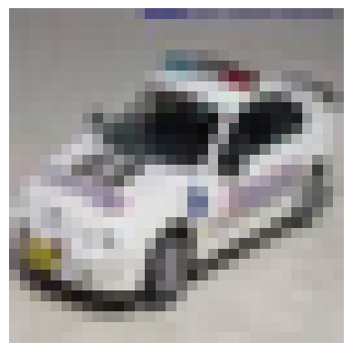
bi = np.random.randint(len(x_test))
plt.imshow(x_test[bi])
plt.axis("off");
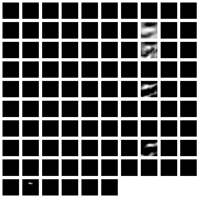
def output_at_layer(X, model, layer_name):
    from tensorflow.keras.models import Model
    return Model(inputs=model.input, outputs=model.get_layer(layer_name).output)(X).numpy()
acts = output_at_layer(x_test[bi:bi+1], model, "conv2d")[0]
acts.shape
(22, 22, 96)
plt.figure(figsize=(10,10))
for i in range(acts.shape[-1]):
    plt.subplot(10,10,i+1)
    plt.imshow(acts[:,:,i], cmap=plt.cm.Greys_r )
    plt.axis("off")
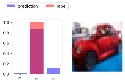
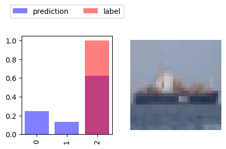
idxs = np.random.permutation(len(x_test))[:5]
preds = model.predict(x_test[idxs])
mlutils.show_preds(x_test[idxs],y_test[idxs], preds)
1/1 ━━━━━━━━━━━━━━━━━━━━ 0s 86ms/step
see
Class activation maps https://jacobgil.github.io/deeplearning/class-activation-maps