3.2 - TF symbolic engine#
!wget -nc --no-cache -O init.py -q https://raw.githubusercontent.com/rramosp/2021.deeplearning/main/content/init.py
import init; init.init(force_download=False);
/content/init.py:2: SyntaxWarning: invalid escape sequence '\S'
  course_id = '\S*deeplearning\S*'
replicating local resources
import numpy as np
import tensorflow as tf
import matplotlib.pyplot as plt
import pandas as pd
%matplotlib inline
%load_ext tensorboard

from sklearn.datasets import *
from local.lib import mlutils
from IPython.display import Image
tf.__version__
'2.19.0'
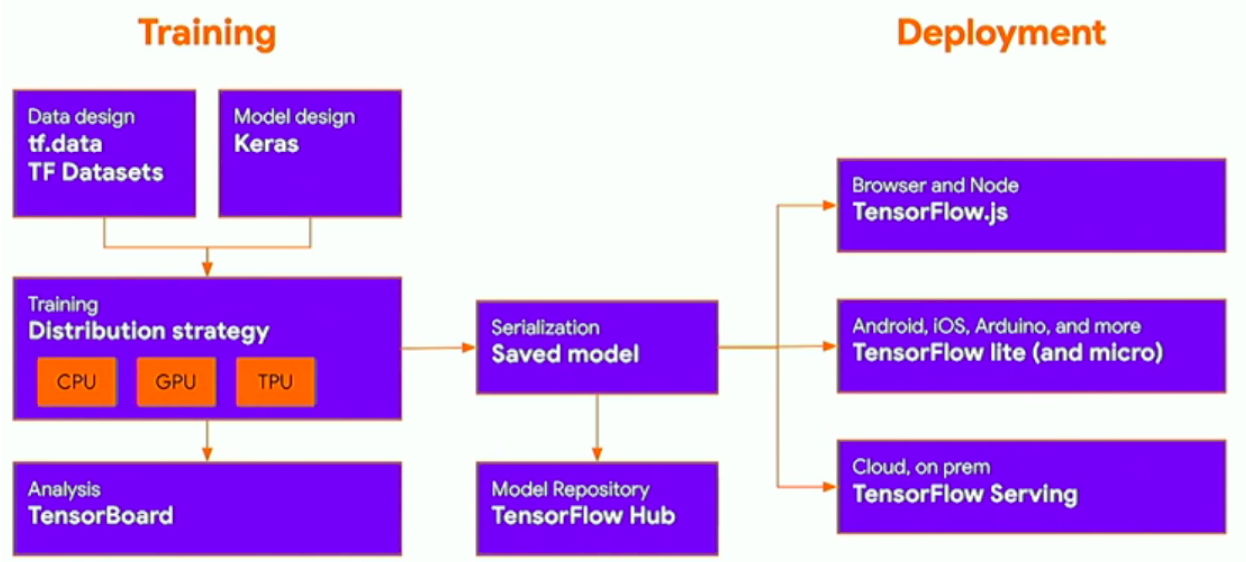
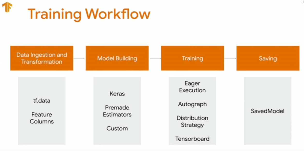
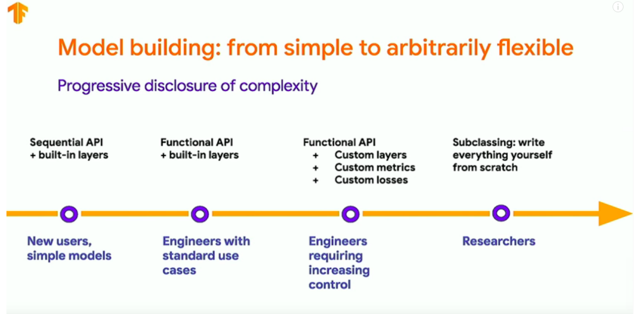
Tensorflow Dev Summit#
the following images are screenshots of the publicly available material from conferences at the TensorFLow Dev Summit
Image("local/imgs/tfCycle.png")
Image("local/imgs/tfTrainingWorkflow.png")
Image("local/imgs/tfAPIs.png")
TF is a symbolic computing + optimization library for machine learning problems#
ML expressions involve:
variables representing data as n-dimensional objects
variables representing parameters as n-dimensional objects
mostly matrix operations (multiplications, convolutions, etc.)
some non linear operations (activation functions)
Recall that in sympy we FIRST define expressions (a computational graph) and THEN we evaluate them feed concrete values.
Tensorflow INTEGRATES both aspects so that building computational graphs LOOKS LIKE writing regular Pytohn code as must as possible.
a
tf.Variablerepresents a symbolic variable, that contains a value
See:
https://www.tensorflow.org/guide/keras/custom_layers_and_models
https://www.tensorflow.org/guide/keras/customizing_what_happens_in_fit
x = tf.Variable(initial_value=[7], name="x", dtype=tf.float32)
y = tf.Variable(initial_value=[9], name="y", dtype=tf.float32)
f = x**2+y**3
f
<tf.Tensor: shape=(1,), dtype=float32, numpy=array([778.], dtype=float32)>
f is SYMBOLIC EXPRESSION (a Tensor in TF terms) that also contains a value attached to it.
for which TF can obtain gradients automatically. This might seem a rather akward way of obtaining the gradient (with GradientTape). The goal is that you write code as in Python and TF takes care of building the computational graph with it.
with tf.GradientTape(persistent=True) as t:
    f = x**2 + y**3

print (t.gradient(f, x), t.gradient(f, y))
tf.Tensor([14.], shape=(1,), dtype=float32) tf.Tensor([243.], shape=(1,), dtype=float32)
print (t.gradient(f, [x,y]))
[<tf.Tensor: shape=(1,), dtype=float32, numpy=array([14.], dtype=float32)>, <tf.Tensor: shape=(1,), dtype=float32, numpy=array([243.], dtype=float32)>]
usually expressions are built within functions decorated with @tf.function for performance
@tf.function
def myf(x,y):
    return x**2 + y**3
with tf.GradientTape(persistent=True) as t:
    f = myf(x,y)

print (t.gradient(f, x), t.gradient(f, y))
tf.Tensor([14.], shape=(1,), dtype=float32) tf.Tensor([243.], shape=(1,), dtype=float32)
!rm -rf logs
mlutils.make_graph(myf, x, y, logdir="logs")
<tensorflow.python.eager.polymorphic_function.polymorphic_function.Function object at 0x7a4c66216030>
%tensorboard --logdir logs
Tensors#
in Tensorflow the notion of a Tensor is just a symbolic multidimensional array. Although, this is a recent simplified version of what always has been known as a tensor in differential geometry (see https://bjlkeng.github.io/posts/tensors-tensors-tensors/).
Observe how Tensorflow naturally deals with multidimensional symbolic variables (Tensors)
n = 3
X = tf.Variable(initial_value=[[2, 6], [3, 1], [4, 5]], name="X", dtype=tf.float32)
w = tf.Variable(initial_value=[[-2],[1]], name="w", dtype=tf.float32)
y = tf.Variable(initial_value=[[8],[2],[3]], name="y", dtype=tf.float32)

with tf.GradientTape(persistent=True) as t:
    f = tf.reduce_mean((tf.matmul(X,w)-y)**2)

g = t.gradient(f, w)
g
<tf.Tensor: shape=(2, 1), dtype=float32, numpy=
array([[-38.      ],
       [-48.666668]], dtype=float32)>
But a tf.Tensor is always a symbolic variable. In order to reconcile symbolic and execution worlds, Tensorflow attaches a value to each symbolic variable, and carries it forward when making derivations.
X,yandware Tensors that we define with a specific valuegis a Tensor derived fromX,yandwthat have ALSO been evaluated with the corresponding values.
g
<tf.Tensor: shape=(2, 1), dtype=float32, numpy=
array([[-38.      ],
       [-48.666668]], dtype=float32)>
g.numpy()
array([[-38.      ],
       [-48.666668]], dtype=float32)
Implementing linear regresion in TF#
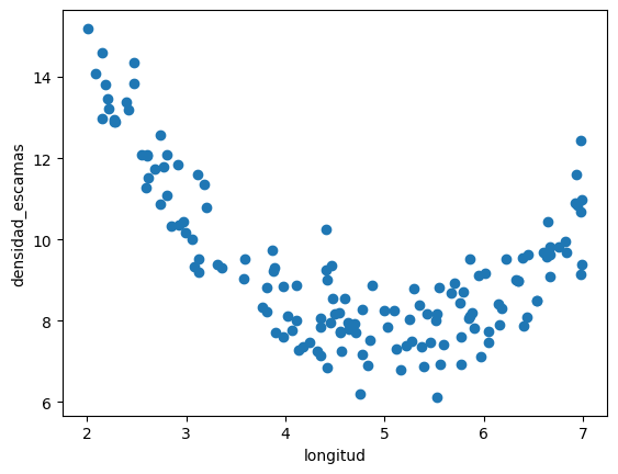
d = pd.read_csv("local/data/trilotropicos.csv")
y = d.densidad_escamas.values.astype(np.float32)
X = np.r_[[d.longitud.values]].T.astype(np.float32)

print(X.shape, y.shape)
plt.scatter(d.longitud, d.densidad_escamas)
plt.xlabel(d.columns[0])
plt.ylabel(d.columns[1]);
(150, 1) (150,)
from sklearn.linear_model import LinearRegression

lr = LinearRegression()
lr.fit(X,y)
lr.coef_, lr.intercept_
(array([-0.71805906], dtype=float32), np.float32(12.689999))
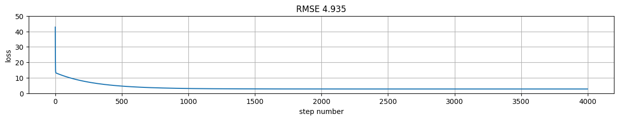
Version 1: raw low level with gradient descent#
beware of typing.
tensorflowis very sensitive to numeric data types (tf.float32,tf.float64, etc.) Default types innumpyandtensorflowmight not always be the same
from progressbar import progressbar as pbar

epochs = 4000
learning_rate = 0.01

# symbolic variables
w = tf.Variable(np.random.normal(size=(X.shape[-1], 1), scale=.6), dtype=tf.float32)
b = tf.Variable(np.random.normal(size=(1,), scale=.6), dtype=tf.float32)
h = []

#optimization loop
for epoch in pbar(range(epochs)):
    with tf.GradientTape() as t:
        preds = tf.matmul(X,w)+b
        loss = tf.reduce_mean( (preds-y.reshape(-1,1))**2)

    gw, gb = t.gradient(loss, [w, b])

    w.assign_sub(learning_rate * gw)
    b.assign_sub(learning_rate * gb)

    h.append([gw.numpy()[0][0], gb.numpy()[0], w.numpy()[0][0], b.numpy()[0], loss.numpy()])
h = np.r_[h]
print (b.numpy(), w.numpy())
100% (4000 of 4000) |####################| Elapsed Time: 0:00:17 Time: 0:00:17
[12.679218] [[-0.7159409]]
rmse = tf.reduce_mean((tf.matmul(X,w)+b-y)**2).numpy()
plt.figure(figsize=(15,2));
plt.plot(h[:,-1]); plt.xlabel("step number"); plt.ylabel("loss"); plt.grid();
plt.title("RMSE %.3f"%rmse);
plt.ylim(0,50)
(0.0, 50.0)
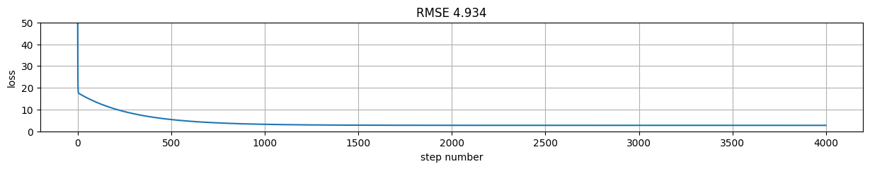
Version 2: using tf.function to speed up#
epochs = 4000

# initialize weights
w.assign(np.random.normal(size=(X.shape[-1],1)).astype(np.float32)*.6)
b.assign(np.random.normal(size=(1,)).astype(np.float32))

@tf.function
def get_gradient(w, b, X, y):
    with tf.GradientTape() as t:
        preds = tf.matmul(X,w)+b
        loss = tf.reduce_mean( (preds-y)**2)

    gw, gb = t.gradient(loss, [w, b])
    return gw, gb, loss

#optimization loop
h = []
for epoch in pbar(range(epochs)):

    gw, gb, loss = get_gradient(w, b, X, y.reshape(-1,1))

    w.assign_sub(learning_rate * gw)
    b.assign_sub(learning_rate * gb)

    h.append([gw.numpy()[0][0], gb.numpy()[0], w.numpy()[0][0], b.numpy()[0], loss.numpy()])
h = np.r_[h]

print (b.numpy(), w.numpy())
100% (4000 of 4000) |####################| Elapsed Time: 0:00:18 Time: 0:00:18
[12.677157] [[-0.7155362]]
predictions = tf.matmul(X,w)+b

rmse = tf.reduce_mean((predictions-y)**2).numpy()
plt.figure(figsize=(15,2));
plt.plot(h[:,-1]); plt.xlabel("step number"); plt.ylabel("loss"); plt.grid();
plt.title("RMSE %.3f"%rmse);
plt.ylim(0,50)
(0.0, 50.0)
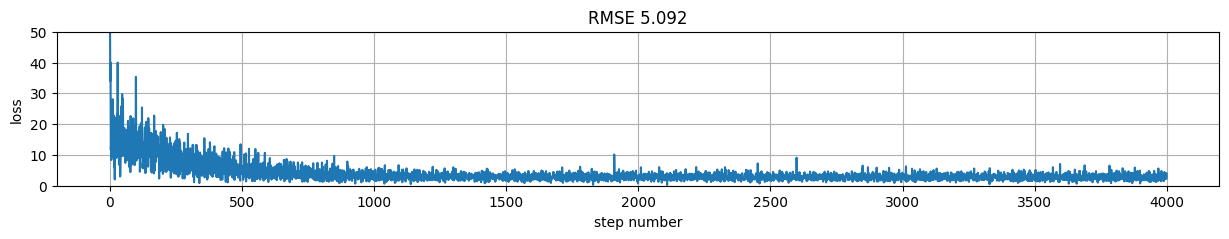
Version 3: using batches with random shuffling (stochastic gradient descent)#
notice we tune the number of epochs as the number of weights updates increases
#optimization loop
batch_size = 16
epochs = 400

# initialize weights
w.assign(np.random.normal(size=(X.shape[-1],1))*.6)
b.assign(np.random.normal(size=(1,)))

h = []

for epoch in pbar(range(epochs)):

    idxs = np.random.permutation(len(X))

    for step in range(len(X)//batch_size+((len(X)%batch_size)!=0)):

        X_batch = X[idxs][step*batch_size:(step+1)*batch_size]
        y_batch = y[idxs][step*batch_size:(step+1)*batch_size]

        gw, gb, loss = get_gradient(w, b, X_batch, y_batch.reshape(-1,1))

        w.assign_sub(learning_rate * gw)
        b.assign_sub(learning_rate * gb)

        h.append([gw.numpy()[0][0], gb.numpy()[0], w.numpy()[0][0], b.numpy()[0], loss.numpy()])
h = np.r_[h]
print (b.numpy(), w.numpy())
100% (400 of 400) |######################| Elapsed Time: 0:00:08 Time: 0:00:08
[12.636945] [[-0.75189483]]
predictions = tf.matmul(X,w)+b

rmse = tf.reduce_mean((predictions-y)**2).numpy()
plt.figure(figsize=(15,2));
plt.plot(h[:,-1]); plt.xlabel("step number"); plt.ylabel("loss"); plt.grid();
plt.title("RMSE %.3f"%rmse);
plt.ylim(0,50)
(0.0, 50.0)
Version 4: packing up with Keras class API and custom SGD#
observe:
the
buildmethod that is called by Keras wheneverinput_shapeis knownwe use
add_weightso that our model weights are known to the Keras model framework (trainable_variables,get_weights, etc.)
see here
class LinearRegressionModel4(tf.keras.Model):

    def build(self, input_shape):
        self.w = self.add_weight(shape=(input_shape[-1], 1), initializer='random_normal',
                                 trainable=True, dtype=tf.float32)

        self.b = self.add_weight(shape=(1,), initializer='random_normal',
                                 trainable=True, dtype=tf.float32)

    def call(self, inputs):
        return tf.matmul(inputs, self.w) + self.b

    @tf.function
    def get_gradient(self, X, y):
        with tf.GradientTape() as t:
            loss = tf.reduce_mean( (self(X)-y)**2)

        gw, gb = t.gradient(loss, [self.w, self.b])
        return gw, gb, loss

    def fit(self, X,y, epochs, batch_size=16, learning_rate=0.01):
        y = y.reshape(-1,1)
        self.h=[]
        for epoch in pbar(range(epochs)):
            idxs = np.random.permutation(len(X))
            for step in range(len(X)//batch_size+((len(X)%batch_size)!=0)):
                X_batch = X[idxs][step*batch_size:(step+1)*batch_size]
                y_batch = y[idxs][step*batch_size:(step+1)*batch_size]

                gw, gb, loss = self.get_gradient(X_batch,y_batch)
                self.w.assign_sub(learning_rate * gw)
                self.b.assign_sub(learning_rate * gb)
                self.h.append([gw.numpy()[0][0], gb.numpy()[0], w.numpy()[0][0], b.numpy()[0], loss.numpy()])
        self.h = np.r_[self.h]
model = LinearRegressionModel4()
observe that we can use the object directly on data to get predictions
model(X[:2])
<tf.Tensor: shape=(2, 1), dtype=float32, numpy=
array([[-0.01385765],
       [ 0.02624173]], dtype=float32)>
or with the .predict method
model.predict(X[:2])
1/1 ━━━━━━━━━━━━━━━━━━━━ 0s 72ms/step
array([[-0.01385765],
       [ 0.02624173]], dtype=float32)
model.trainable_variables
[<Variable path=linear_regression_model4/variable, shape=(1, 1), dtype=float32, value=[[-0.02411834]]>,
 <Variable path=linear_regression_model4/variable_1, shape=(1,), dtype=float32, value=[0.07820677]>]
model.get_weights()
[array([[-0.02411834]], dtype=float32), array([0.07820677], dtype=float32)]
and fit the model
model.fit(X, y, epochs=400, batch_size=16)
100% (400 of 400) |######################| Elapsed Time: 0:00:09 Time: 0:00:09
model.b.numpy(), model.w.numpy()
(array([12.672345], dtype=float32), array([[-0.7251613]], dtype=float32))
predictions = model(X)

rmse = tf.reduce_mean((predictions-y)**2).numpy()
plt.figure(figsize=(15,2));
plt.plot(model.h[:,-1]); plt.xlabel("step number"); plt.ylabel("loss"); plt.grid();
plt.title("RMSE %.3f"%rmse);
plt.ylim(0,50)
(0.0, 50.0)

Version 5: Sequential Keras model with standard loop#
from tensorflow.keras import Sequential
from tensorflow.keras.layers import Dense

def get_model5():
    model = Sequential()
    model.add(Dense(1, input_shape=(X.shape[-1],), activation="linear"))
    model.compile(optimizer=tf.keras.optimizers.SGD(learning_rate=0.01),
                  metrics=["mean_absolute_error"],
                  loss="mse")
# equivalent forms for loss
#                  loss = lambda y_true, y_pred: tf.reduce_mean((y_true-y_pred)**2))
#                  loss="mean_squared_error")
#                  loss=tf.keras.metrics.mean_squared_error)
    return model
from sklearn.model_selection import train_test_split
X_train, X_val, y_train, y_val = train_test_split(X,y.reshape(-1,1), test_size=0.2)
X_train.shape, X_val.shape, y_train.shape, y_val.shape
((120, 1), (30, 1), (120, 1), (30, 1))
!rm -rf logs
model = get_model5()

tb_callback = tf.keras.callbacks.TensorBoard('./logs', update_freq=1)
model.fit(X_train,y_train, epochs=100, batch_size=5, verbose=0,
          callbacks=[tb_callback], validation_data=(X_val, y_val))

model.weights
/usr/local/lib/python3.12/dist-packages/keras/src/layers/core/dense.py:93: UserWarning: Do not pass an `input_shape`/`input_dim` argument to a layer. When using Sequential models, prefer using an `Input(shape)` object as the first layer in the model instead.
  super().__init__(activity_regularizer=activity_regularizer, **kwargs)
[<Variable path=sequential/dense/kernel, shape=(1, 1), dtype=float32, value=[[-0.63442165]]>,
 <Variable path=sequential/dense/bias, shape=(1,), dtype=float32, value=[12.918131]>]
history is now logged only per epoch
model.history.history.keys()
dict_keys(['loss', 'mean_absolute_error', 'val_loss', 'val_mean_absolute_error'])
predictions = model(X)
rmse = np.mean((predictions-y)**2)
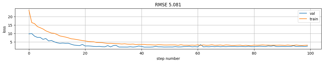
plt.figure(figsize=(15,2));
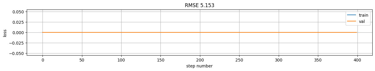
plt.plot(model.history.history["val_loss"], label="val");
plt.plot(model.history.history["loss"], label="train");
plt.xlabel("step number"); plt.ylabel("loss"); plt.grid();
plt.title("RMSE %.3f"%rmse); plt.legend();
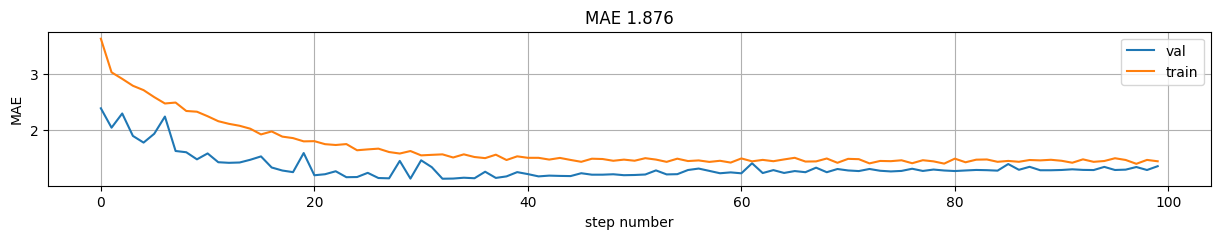
mae = np.mean(np.abs(predictions-y))

plt.figure(figsize=(15,2));
plt.plot(model.history.history["val_mean_absolute_error"], label="val");
plt.plot(model.history.history["mean_absolute_error"], label="train");
plt.xlabel("step number"); plt.ylabel("MAE"); plt.grid();
plt.title("MAE %.3f"%mae); plt.legend();
%tensorboard --logdir logs
Version 6: Custom model with Keras class API and standard loop#
class LinearRegressionModel6(tf.keras.Model):

    def build(self, input_shape):
        self.w = self.add_weight(shape=(input_shape[-1], 1),
                                 initializer='random_normal',
                                 trainable=True, dtype=np.float32)

        self.b = self.add_weight(shape=(1,),
                                 initializer='random_normal',
                                 trainable=True, dtype=np.float32)

    def call(self, inputs):
        return tf.matmul(inputs, self.w) + self.b
model = LinearRegressionModel6()
!rm -rf logs
model = LinearRegressionModel6()
model.compile(optimizer=tf.keras.optimizers.SGD(learning_rate=0.02),
           loss="mse", metrics=['mean_absolute_error'])

tb_callback = tf.keras.callbacks.TensorBoard('./logs', update_freq=1)


model.fit(X_train,y_train, epochs=100, batch_size=5, callbacks=[tb_callback],
       verbose=0, validation_data=(X_val, y_val))
<keras.src.callbacks.history.History at 0x7a4bd84d6000>
model.b.numpy(), model.w.numpy()[0]
(array([13.135199], dtype=float32), array([-0.7534032], dtype=float32))
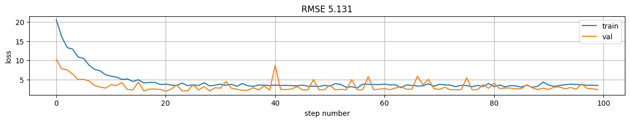
predictions = model(X)
rmse = np.mean((predictions-y)**2)

plt.figure(figsize=(15,2));
plt.plot(model.history.history["loss"], label="train");
plt.plot(model.history.history["val_loss"], label="val");
plt.xlabel("step number"); plt.ylabel("loss"); plt.grid();
plt.title("RMSE %.3f"%rmse); plt.legend();
Version 7: Using train_step \(\rightarrow\) control loss and gradients on a custom model.#
class LinearRegressionModel7(tf.keras.Model):

    def build(self, input_shape):
        self.w = self.add_weight(shape=(input_shape[-1], 1),
                                 initializer='random_normal',
                                 trainable=True, dtype=np.float32)

        self.b = self.add_weight(shape=(1,),
                                 initializer='random_normal',
                                 trainable=True, dtype=np.float32)

        self.loss_fn = tf.keras.metrics.MeanSquaredError()

    def call(self, inputs):
        return tf.matmul(inputs, self.w) + self.b

    def test_step(self, data):
        # here we implement loss by hand
        return {'loss': tf.reduce_mean((self(X)-y)**2)  }

    @tf.function
    def train_step(self, data):
        X,y = data
        loss_fn = lambda y_true, y_preds: tf.reduce_mean((y_true-y_preds)**2)
        with tf.GradientTape() as tape:
            # we use tf.keras loss function (equivalent to test_step)
            loss_fn = tf.keras.metrics.MSE
            loss = tf.reduce_mean(loss_fn(y, self(X)))

        grads = tape.gradient(loss, self.trainable_variables)
        self.optimizer.apply_gradients(zip(grads, self.trainable_variables))

        return {'loss': loss}
model = LinearRegressionModel7()
model.compile(optimizer=tf.keras.optimizers.SGD(learning_rate=0.02))
#model.compile(optimizer=tf.keras.optimizers.Adam(learning_rate=0.035))
model.fit(X_train,y_train, epochs=400, batch_size=5, verbose=0, validation_data=(X_val, y_val))
<keras.src.callbacks.history.History at 0x7a4bd8e636e0>
[i.numpy() for i in model.trainable_variables]
[array([[-0.9850567]], dtype=float32), array([13.005241], dtype=float32)]
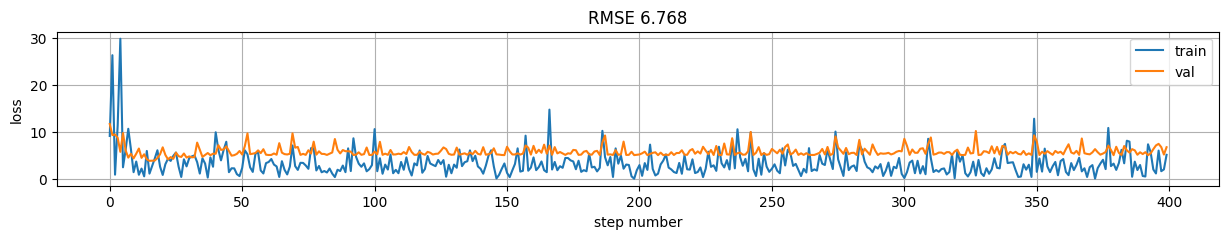
predictions = model(X)
rmse = np.mean((predictions-y)**2)

plt.figure(figsize=(15,2));
plt.plot(model.history.history["loss"], label="train");
plt.plot(model.history.history["val_loss"], label="val");
plt.xlabel("step number"); plt.ylabel("loss"); plt.grid();
plt.title("RMSE %.3f"%rmse); plt.legend();
Version 8: Using train_step \(\rightarrow\) control loss and gradients on a standard model.#
observe that:
we use a standard
Denselayer,we use a custom loss function and
optimizer.apply_gradients
class CustomModel(tf.keras.Model):

    def test_step(self, data):
        X,y = data
        return {'loss': tf.reduce_mean((self(X)-y)**2)}

    @tf.function
    def train_step(self, data):
        X,y = data

        with tf.GradientTape() as tape:
            y_pred = self(X, training=True)
            loss_value = tf.reduce_mean((y_pred-y)**2)

        grads = tape.gradient(loss_value, self.trainable_variables)
        self.optimizer.apply_gradients(zip(grads, self.trainable_variables))

        return {'loss': loss_value}
from tensorflow.keras.layers import Dense, Input

def get_model8():

    inputs = tf.keras.layers.Input(shape=(1,))
    outputs = tf.keras.layers.Dense(1, activation="linear")(inputs)

    model = CustomModel(inputs, outputs)

    model.compile(optimizer=tf.keras.optimizers.SGD(learning_rate=0.02))
    return model
our custom loop (for any model !!!)
model = get_model8()
model.summary()
Model: "custom_model_2"
┏━━━━━━━━━━━━━━━━━━━━━━━━━━━━━━━━━┳━━━━━━━━━━━━━━━━━━━━━━━━┳━━━━━━━━━━━━━━━┓
┃ Layer (type)                    ┃ Output Shape           ┃       Param # ┃
┡━━━━━━━━━━━━━━━━━━━━━━━━━━━━━━━━━╇━━━━━━━━━━━━━━━━━━━━━━━━╇━━━━━━━━━━━━━━━┩
│ input_layer_4 (InputLayer)      │ (None, 1)              │             0 │
├─────────────────────────────────┼────────────────────────┼───────────────┤
│ dense_3 (Dense)                 │ (None, 1)              │             2 │
└─────────────────────────────────┴────────────────────────┴───────────────┘
Total params: 2 (8.00 B)
Trainable params: 2 (8.00 B)
Non-trainable params: 0 (0.00 B)
model.weights
[<Variable path=dense_3/kernel, shape=(1, 1), dtype=float32, value=[[-1.709459]]>,
 <Variable path=dense_3/bias, shape=(1,), dtype=float32, value=[0.]>]
model.trainable_variables
[<Variable path=dense_3/kernel, shape=(1, 1), dtype=float32, value=[[-1.709459]]>,
 <Variable path=dense_3/bias, shape=(1,), dtype=float32, value=[0.]>]
model.fit(X_train,y_train.reshape(-1,1), epochs=40, batch_size=5, verbose=0, validation_data=(X_val, y_val))
<keras.src.callbacks.history.History at 0x7a4bd8c86000>
model.trainable_variables
[<Variable path=dense_3/kernel, shape=(1, 1), dtype=float32, value=[[-0.73976785]]>,
 <Variable path=dense_3/bias, shape=(1,), dtype=float32, value=[13.170137]>]
predictions = model(X)
rmse = np.mean((predictions-y)**2)

plt.figure(figsize=(15,2));
plt.plot(model.history.history["loss"], label="train");
plt.plot(model.history.history["val_loss"], label="val");
plt.xlabel("step number"); plt.ylabel("loss"); plt.grid();
plt.title("RMSE %.3f"%rmse); plt.legend();