4.9 - Atrous convolutions#
!wget -nc --no-cache -O init.py -q https://raw.githubusercontent.com/rramosp/2021.deeplearning/main/content/init.py
import init; init.init(force_download=False);
import numpy as np
import tensorflow as tf
import matplotlib.pyplot as plt
import pandas as pd
%matplotlib inline
print (tf.__version__)

def dilate(simg):
    k = simg.copy()
    for i in range(k.shape[1]-1):
        k = np.insert(k, 1+2*i, values=0, axis=1)
    for i in range(k.shape[0]-1):
        k = np.insert(k, 1+2*i, values=0, axis=0)
    return k
2.4.1
See Types of convolutions for a global view of how convolutions can be made in different ways.
Atrous convolutions are done through dilation on the filter (not on the image as in transposed convolutions)
This is implemented in the same Conv2D layer through the dilation_rate argument.
The goal is that with the same filter, one could capture a larger receptive field and thus, doing an operation at a smaller resolution while keeping some detail.
simg = np.r_[[[4,5,8,7],[1,8,8,8],[3,6,6,4],[6,5,7,8]]].astype(np.float32)
kernel = np.r_[[[10,-8],[15,-2]]]
ddkernel = dilate(kernel)
print ("filter\n", kernel)
print ("dilated filter\n", ddkernel)
filter
 [[10 -8]
 [15 -2]]
dilated filter
 [[10  0 -8]
 [ 0  0  0]
 [15  0 -2]]
regular convolution
c1 = tf.keras.layers.Conv2D(filters=1, kernel_size=kernel.shape, padding="VALID", activation="linear")
c1.build(input_shape=[None, *simg[:,:,None].shape])
c1.set_weights([kernel.T[:,:,None, None], np.r_[0]])
c1(simg.T[None, :, :, None]).numpy().T[0,:,:,0]
array([[ -1.,  90., 128.],
       [-21.,  94.,  98.],
       [ 62.,  73., 117.]], dtype=float32)
dilated convolution
c1 = tf.keras.layers.Conv2D(filters=1, kernel_size=ddkernel.shape, padding="VALID", activation="linear")
c1.build(input_shape=[None, *simg[:,:,None].shape])
c1.set_weights([ddkernel.T[:,:,None, None], np.r_[0]])
c1(simg.T[None, :, :, None]).numpy().T[0,:,:,0]
array([[ 9., 76.],
       [22., 75.]], dtype=float32)
observe how the receptive field of the dilated filter (3z3) is larger than the original filter (2x2)
(simg[:2,:2]*kernel).sum() # corresponds to the (0,0) regular convolution output
-1.0
(simg[:3,:3]*ddkernel).sum() # corresponds to the (0,0) dilated convolution output
9.0
observe we obtain the same result by using dilation_rate=1
c1 = tf.keras.layers.Conv2D(filters=1, kernel_size=ddkernel.shape, padding="VALID", activation="linear")
c1.build(input_shape=[None, *simg[:,:,None].shape])
c1.set_weights([ddkernel.T[:,:,None, None], np.r_[0]])
c1(simg.T[None, :, :, None]).numpy().T[0,:,:,0]
array([[ 9., 76.],
       [22., 75.]], dtype=float32)
simg
array([[4., 5., 8., 7.],
       [1., 8., 8., 8.],
       [3., 6., 6., 4.],
       [6., 5., 7., 8.]], dtype=float32)
Intuition#
somehow, with atrous convolutions we are using a lower resolution filter at a higher resolution image, with the hope to extract semantic content while keeping some details
from skimage import io
img = io.imread("local/imgs/sample_img.png")
img = (img-np.min(img))/(np.max(img)-np.min(img))
img = img.reshape(1,*img.shape, 1)
f = np.r_[[-1., -1.,  1., -1., -1., -1., -1.,  1.,  1.],
          [ 1., -1.,  1., -1., -1.,  1., -1., -1., -1.]].reshape(3,3,1,2)
plt.figure(figsize=(5,2))
plt.subplot(131);  plt.imshow(img[0,:,:,0], cmap=plt.cm.Greys_r); plt.axis("off")
plt.subplot(132);  plt.imshow(f[:,:,0,0]); plt.axis("off")
plt.subplot(133);  plt.imshow(f[:,:,0,1]); plt.axis("off");

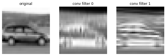
observe the regular convolution at the original resolution
c = tf.keras.layers.Conv2D(filters=f.shape[-1], kernel_size=f.shape[:2], activation="sigmoid", padding='VALID', dtype=tf.float64)
c.build(input_shape=(1,7,7,f.shape[2]))   # any shape would do here, just initializing weights
c.set_weights([f, np.zeros(2)])
cimg = c(img).numpy()
print (cimg.shape)
plt.figure(figsize=(10,6))
plt.subplot(131); plt.imshow(img[0,:,:,0], cmap=plt.cm.Greys_r); plt.axis("off"); plt.title("original")
plt.subplot(132); plt.imshow(cimg[0,:,:,0], cmap=plt.cm.Greys_r); plt.axis("off"); plt.title("conv filter 0")
plt.subplot(133); plt.imshow(cimg[0,:,:,1], cmap=plt.cm.Greys_r); plt.axis("off"); plt.title("conv filter 1")
(1, 30, 30, 2)
Text(0.5, 1.0, 'conv filter 1')
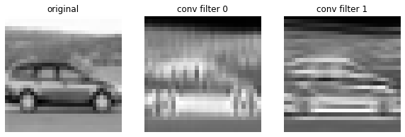
now a dilated convolution, think of applying the same filter at a lower resolution while keeping details
c = tf.keras.layers.Conv2D(filters=f.shape[-1], kernel_size=f.shape[:2],
                           dilation_rate=2,
                           activation="sigmoid", padding='VALID', dtype=tf.float64)
c.build(input_shape=(1,7,7,f.shape[2]))   # any shape would do here, just initializing weights
c.set_weights([f, np.zeros(2)])
cimg = c(img).numpy()
print (cimg.shape)

plt.figure(figsize=(10,6))
plt.subplot(131); plt.imshow(img[0,:,:,0], cmap=plt.cm.Greys_r); plt.axis("off"); plt.title("original")
plt.subplot(132); plt.imshow(cimg[0,:,:,0], cmap=plt.cm.Greys_r); plt.axis("off"); plt.title("conv filter 0")
plt.subplot(133); plt.imshow(cimg[0,:,:,1], cmap=plt.cm.Greys_r); plt.axis("off"); plt.title("conv filter 1")
(1, 28, 28, 2)
Text(0.5, 1.0, 'conv filter 1')
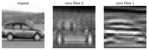
now we actually resize the image and THEN apply the original filter (with no dilution), so that the final resolution is the same
However, observe how the previous dilated convolutions tries to keep sharper details of the original image
from skimage.transform import resize
n = 30
simg = resize(img[0,:,:,0], (n, n)).reshape(1,n,n,1)
simg.shape
(1, 30, 30, 1)
c = tf.keras.layers.Conv2D(filters=f.shape[-1], kernel_size=f.shape[:2], activation="sigmoid", padding='VALID', dtype=tf.float64)
c.build(input_shape=(1,7,7,f.shape[2]))   # any shape would do here, just initializing weights
c.set_weights([f, np.zeros(2)])
csimg = c(simg).numpy()
print(csimg.shape)

plt.figure(figsize=(10,6))
plt.subplot(131); plt.imshow(simg[0,:,:,0], cmap=plt.cm.Greys_r); plt.axis("off"); plt.title("original")
plt.subplot(132); plt.imshow(csimg[0,:,:,0], cmap=plt.cm.Greys_r); plt.axis("off"); plt.title("conv filter 0")
plt.subplot(133); plt.imshow(csimg[0,:,:,1], cmap=plt.cm.Greys_r); plt.axis("off"); plt.title("conv filter 1")
(1, 28, 28, 2)
Text(0.5, 1.0, 'conv filter 1')