
5.2 LSTM and GRU#
!wget -nc --no-cache -O init.py -q https://raw.githubusercontent.com/rramosp/2021.deeplearning/main/content/init.py
import init; init.init(force_download=False);
%matplotlib inline
U5.02 - Long Short Term Memory RNN#
The main drawback of conventional RNNs is its inability to learn long term dependency, or even the capacity of capturing long and short dependences at the same time.
Remenber that in a RNN:
and,
and,
Therefore, during the training phase of one time series, the matrix \(\bf{V}\), which contains the weights of the feedback loop, mulplies by itself \((\tau-1)\) times. Thus, if its values are close to zero, the weights end up vanishing. On the contrary, if the weights of \(\bf{V}\) are to large, they end up diverging (in case of no regularization method be included). This fact makes conventional RNNs very unstable.
They are also very sensitive to vanishing gradients phenomena, but it can be overcome by using Relu or LeakyRelu activation functions.
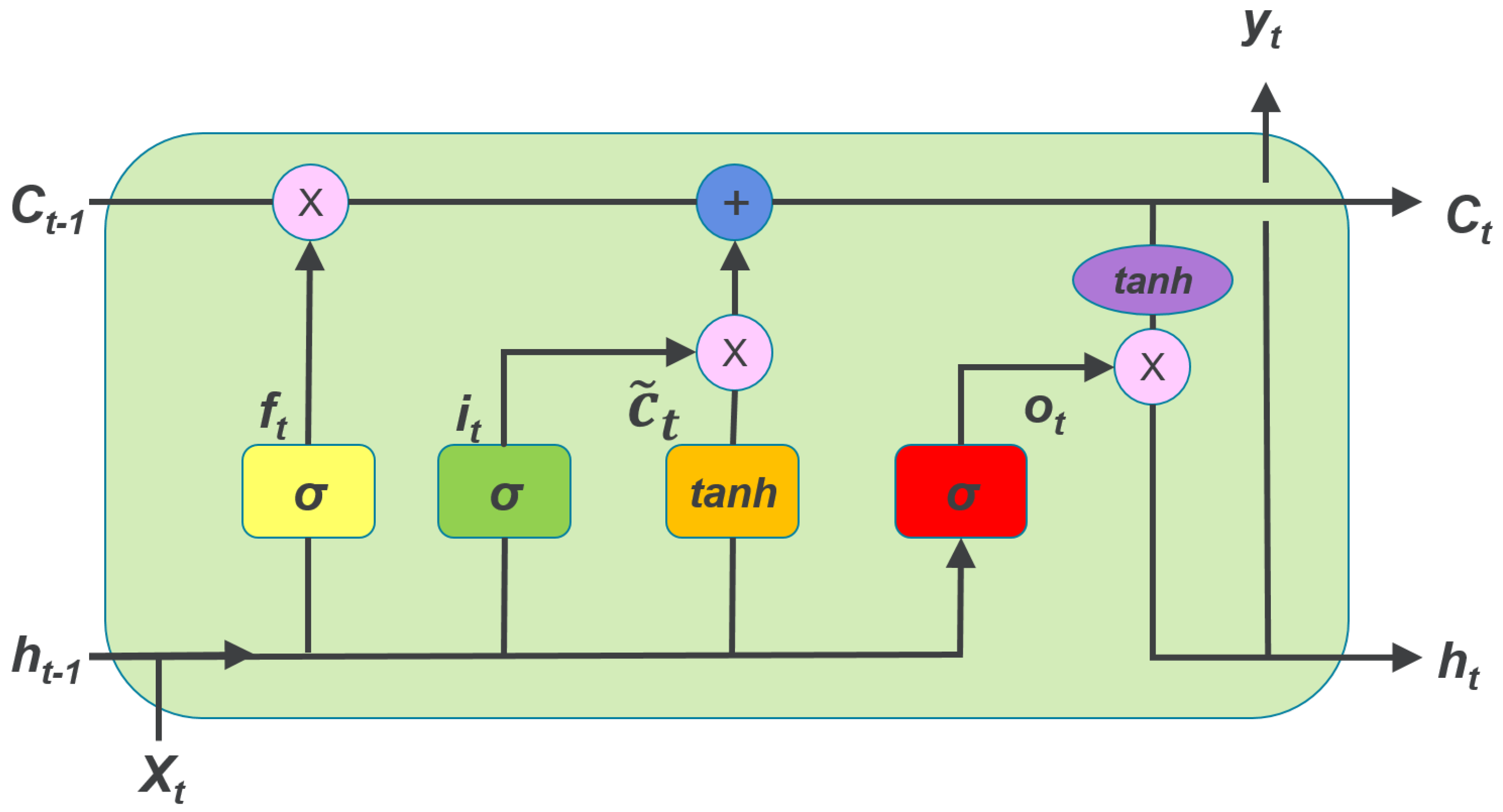
LSTMs are a type of RNNs proposed to takle the former problems. They were introduced in 1997 and are based on different type of basic unit called cell.
from IPython.display import Image
Image(filename='local/imgs/LSTM2.png', width=1200)
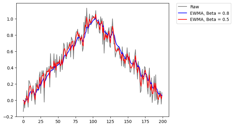
The cells use the principle of cumulative average called Exponential Weighted Moving Average (EWMA) originally proposed for a type of units called leaky units. EWMA takes into account more or less information from the past based on a \(\beta\) paratemer. The rule is given by: \(\mu^{(t)} \leftarrow \beta \mu^{(t-1)} + (1 - \beta)\upsilon^{(t)}\).
import numpy as np
import matplotlib.pyplot as plt
# make a hat function, and add noise
x = np.linspace(0,1,100)
x = np.hstack((x,x[::-1]))
x += np.random.normal( loc=0, scale=0.1, size=200 )
plt.plot( x, 'k', alpha=0.5, label='Raw' )

Beta1 = 0.8
Beta2 = 0.5
x1 = np.zeros(200)
x2 = np.copy(x1)
for i in range(1,200):
    x1[i] = Beta1*x1[i-1] + (1-Beta1)*x[i]
    x2[i] = Beta2*x2[i-1] + (1-Beta2)*x[i]
# regular EWMA, with bias against trend
plt.plot( x1, 'b', label='EWMA, Beta = 0.8' )

# "corrected" (?) EWMA
plt.plot( x2, 'r', label='EWMA, Beta = 0.5' )

plt.legend(bbox_to_anchor=(1.05, 1), loc=2, borderaxespad=0.)
plt.show()
#savefig( 'ewma_correction.png', fmt='png', dpi=100 )
The LSTM network uses the same principle the level of memory or time dependence, but instead of one controling parameter, it define gates adjusted during the training phase.
Every cell LSTM contains three gates (the three \(\sigma's\) in the former graph):
The first step in the LSTM is to decide what information is going to be throwed away from the cell state. This decision is made by a sigmoid layer called the forget gate layer. It looks at \(h_{t−1}\) and \(x_t\), and outputs a number between 0 and 1 for each number in the cell state \(C_{t−1}\). A 1 represents “completely keep this” while a 0 represents “completely get rid of this.”
The next step is to decide what new information is going to be stored in the cell state. This has two parts. First, a sigmoid layer called the input gate layer decides which values will be updated. Next, a tanh layer creates a vector of new candidate values, \(\tilde{C}_t\), that could be added to the state.
Finally, the cell decides what is going to output. This output will be based on the cell state, but will be a filtered version. First, it runs a output gate layer which decides what part of the cell state is going to output. Then, the cell state is passed through a tanh function (to push the values to be between −1 and 1) and multiplied it by the output of the gate.
Based on these gates, the state of the cell and output of the cell can be calculated as:
Image(filename='local/imgs/LSTM2.jpeg', width=1200)
# Importing the libraries
import numpy as np
import matplotlib.pyplot as plt
plt.style.use('fivethirtyeight')
import pandas as pd
from sklearn.preprocessing import MinMaxScaler
from tensorflow.keras.models import Sequential
from tensorflow.keras.layers import Dense, LSTM, Dropout, GRU, SimpleRNN, Input
import math
from sklearn.metrics import mean_squared_error
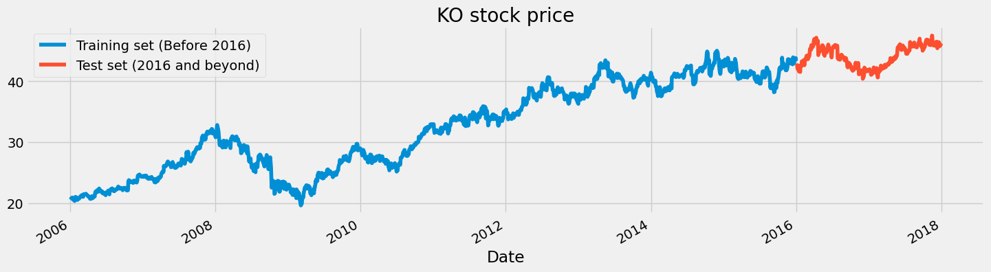
# First, we get the data
dataset = pd.read_csv('local/data/KO_2006-01-01_to_2018-01-01.csv', index_col='Date', parse_dates=['Date'])
dataset.head()
| Open | High | Low | Close | Volume | Name | |
|---|---|---|---|---|---|---|
| Date | ||||||
| 2006-01-03 | 20.40 | 20.50 | 20.18 | 20.45 | 13640800 | KO |
| 2006-01-04 | 20.50 | 20.54 | 20.33 | 20.41 | 19993200 | KO |
| 2006-01-05 | 20.36 | 20.56 | 20.29 | 20.51 | 16613400 | KO |
| 2006-01-06 | 20.53 | 20.78 | 20.43 | 20.70 | 17122800 | KO |
| 2006-01-09 | 20.74 | 20.84 | 20.62 | 20.80 | 13819800 | KO |
# Checking for missing values
training_set = dataset[:'2015'].iloc[:,1:2].values
test_set = dataset['2016':].iloc[:,1:2].values
test_set[np.isnan(test_set)] = dataset['High'].max()
# We have chosen 'High' attribute for prices. Let's see what it looks like
dataset["High"][:'2015'].plot(figsize=(16,4),legend=True)
dataset["High"]['2016':].plot(figsize=(16,4),legend=True)
plt.legend(['Training set (Before 2016)','Test set (2016 and beyond)'])
plt.title('KO stock price')
plt.show()
# Scaling the training set
sc = MinMaxScaler(feature_range=(0,1))
training_set_scaled = sc.fit_transform(training_set)
from local.lib.DataPreparationRNN import create_dataset
look_back = 10
X_train, y_train = create_dataset(training_set_scaled, look_back)
print(X_train.shape)
print(y_train.shape)
(2507, 10)
(2507,)
# The RNN architecture
model = Sequential()
model.add(Input(shape=(X_train.shape[1],1)))
# First RNN layer with Dropout regularisation
model.add(SimpleRNN(units=50))
model.add(Dropout(0.2))
# The output layer
model.add(Dense(units=1))
model.summary()
Model: "sequential"
┏━━━━━━━━━━━━━━━━━━━━━━━━━━━━━━━━━┳━━━━━━━━━━━━━━━━━━━━━━━━┳━━━━━━━━━━━━━━━┓
┃ Layer (type)                    ┃ Output Shape           ┃       Param # ┃
┡━━━━━━━━━━━━━━━━━━━━━━━━━━━━━━━━━╇━━━━━━━━━━━━━━━━━━━━━━━━╇━━━━━━━━━━━━━━━┩
│ simple_rnn (SimpleRNN)          │ (None, 50)             │         2,600 │
├─────────────────────────────────┼────────────────────────┼───────────────┤
│ dropout (Dropout)               │ (None, 50)             │             0 │
├─────────────────────────────────┼────────────────────────┼───────────────┤
│ dense (Dense)                   │ (None, 1)              │            51 │
└─────────────────────────────────┴────────────────────────┴───────────────┘
Total params: 2,651 (10.36 KB)
Trainable params: 2,651 (10.36 KB)
Non-trainable params: 0 (0.00 B)
Let’s remember what a RNN can do:
# Compiling the RNN
model.compile(optimizer='adam',loss='mean_squared_error')
# Fitting to the training set
model.fit(X_train.reshape(X_train.shape[0],look_back,1),y_train,epochs=50,batch_size=32)
Epoch 1/50
79/79 ━━━━━━━━━━━━━━━━━━━━ 0s 657us/step - loss: 0.0611
Epoch 2/50
79/79 ━━━━━━━━━━━━━━━━━━━━ 0s 562us/step - loss: 0.0064
Epoch 3/50
79/79 ━━━━━━━━━━━━━━━━━━━━ 0s 563us/step - loss: 0.0046
Epoch 4/50
79/79 ━━━━━━━━━━━━━━━━━━━━ 0s 563us/step - loss: 0.0040
Epoch 5/50
79/79 ━━━━━━━━━━━━━━━━━━━━ 0s 570us/step - loss: 0.0035
Epoch 6/50
79/79 ━━━━━━━━━━━━━━━━━━━━ 0s 563us/step - loss: 0.0030
Epoch 7/50
79/79 ━━━━━━━━━━━━━━━━━━━━ 0s 559us/step - loss: 0.0029
Epoch 8/50
79/79 ━━━━━━━━━━━━━━━━━━━━ 0s 561us/step - loss: 0.0027
Epoch 9/50
79/79 ━━━━━━━━━━━━━━━━━━━━ 0s 559us/step - loss: 0.0026
Epoch 10/50
79/79 ━━━━━━━━━━━━━━━━━━━━ 0s 558us/step - loss: 0.0026
Epoch 11/50
79/79 ━━━━━━━━━━━━━━━━━━━━ 0s 560us/step - loss: 0.0025
Epoch 12/50
79/79 ━━━━━━━━━━━━━━━━━━━━ 0s 559us/step - loss: 0.0021
Epoch 13/50
79/79 ━━━━━━━━━━━━━━━━━━━━ 0s 562us/step - loss: 0.0020
Epoch 14/50
79/79 ━━━━━━━━━━━━━━━━━━━━ 0s 559us/step - loss: 0.0019
Epoch 15/50
79/79 ━━━━━━━━━━━━━━━━━━━━ 0s 563us/step - loss: 0.0022
Epoch 16/50
79/79 ━━━━━━━━━━━━━━━━━━━━ 0s 566us/step - loss: 0.0019
Epoch 17/50
79/79 ━━━━━━━━━━━━━━━━━━━━ 0s 560us/step - loss: 0.0022
Epoch 18/50
79/79 ━━━━━━━━━━━━━━━━━━━━ 0s 561us/step - loss: 0.0019
Epoch 19/50
79/79 ━━━━━━━━━━━━━━━━━━━━ 0s 588us/step - loss: 0.0020
Epoch 20/50
79/79 ━━━━━━━━━━━━━━━━━━━━ 0s 584us/step - loss: 0.0019
Epoch 21/50
79/79 ━━━━━━━━━━━━━━━━━━━━ 0s 577us/step - loss: 0.0016
Epoch 22/50
79/79 ━━━━━━━━━━━━━━━━━━━━ 0s 582us/step - loss: 0.0019
Epoch 23/50
79/79 ━━━━━━━━━━━━━━━━━━━━ 0s 572us/step - loss: 0.0016
Epoch 24/50
79/79 ━━━━━━━━━━━━━━━━━━━━ 0s 584us/step - loss: 0.0017
Epoch 25/50
79/79 ━━━━━━━━━━━━━━━━━━━━ 0s 597us/step - loss: 0.0016
Epoch 26/50
79/79 ━━━━━━━━━━━━━━━━━━━━ 0s 589us/step - loss: 0.0015
Epoch 27/50
79/79 ━━━━━━━━━━━━━━━━━━━━ 0s 579us/step - loss: 0.0016
Epoch 28/50
79/79 ━━━━━━━━━━━━━━━━━━━━ 0s 883us/step - loss: 0.0016
Epoch 29/50
79/79 ━━━━━━━━━━━━━━━━━━━━ 0s 593us/step - loss: 0.0014
Epoch 30/50
79/79 ━━━━━━━━━━━━━━━━━━━━ 0s 616us/step - loss: 0.0013
Epoch 31/50
79/79 ━━━━━━━━━━━━━━━━━━━━ 0s 614us/step - loss: 0.0013
Epoch 32/50
79/79 ━━━━━━━━━━━━━━━━━━━━ 0s 649us/step - loss: 0.0012
Epoch 33/50
79/79 ━━━━━━━━━━━━━━━━━━━━ 0s 641us/step - loss: 0.0012
Epoch 34/50
79/79 ━━━━━━━━━━━━━━━━━━━━ 0s 617us/step - loss: 0.0012
Epoch 35/50
79/79 ━━━━━━━━━━━━━━━━━━━━ 0s 632us/step - loss: 0.0011
Epoch 36/50
79/79 ━━━━━━━━━━━━━━━━━━━━ 0s 635us/step - loss: 0.0011
Epoch 37/50
79/79 ━━━━━━━━━━━━━━━━━━━━ 0s 635us/step - loss: 9.8205e-04
Epoch 38/50
79/79 ━━━━━━━━━━━━━━━━━━━━ 0s 616us/step - loss: 0.0012
Epoch 39/50
79/79 ━━━━━━━━━━━━━━━━━━━━ 0s 612us/step - loss: 9.8427e-04
Epoch 40/50
79/79 ━━━━━━━━━━━━━━━━━━━━ 0s 612us/step - loss: 0.0010
Epoch 41/50
79/79 ━━━━━━━━━━━━━━━━━━━━ 0s 622us/step - loss: 0.0010
Epoch 42/50
79/79 ━━━━━━━━━━━━━━━━━━━━ 0s 622us/step - loss: 9.7476e-04
Epoch 43/50
79/79 ━━━━━━━━━━━━━━━━━━━━ 0s 618us/step - loss: 9.1240e-04
Epoch 44/50
79/79 ━━━━━━━━━━━━━━━━━━━━ 0s 633us/step - loss: 0.0011
Epoch 45/50
79/79 ━━━━━━━━━━━━━━━━━━━━ 0s 645us/step - loss: 8.2203e-04
Epoch 46/50
79/79 ━━━━━━━━━━━━━━━━━━━━ 0s 648us/step - loss: 9.9008e-04
Epoch 47/50
79/79 ━━━━━━━━━━━━━━━━━━━━ 0s 627us/step - loss: 8.7365e-04
Epoch 48/50
79/79 ━━━━━━━━━━━━━━━━━━━━ 0s 955us/step - loss: 9.1499e-04
Epoch 49/50
79/79 ━━━━━━━━━━━━━━━━━━━━ 0s 627us/step - loss: 9.0956e-04
Epoch 50/50
79/79 ━━━━━━━━━━━━━━━━━━━━ 0s 640us/step - loss: 8.3333e-04
<keras.src.callbacks.history.History at 0x32b78d6a0>
dataset_total = pd.concat((dataset["High"][:'2016'],dataset["High"]['2017':]),axis=0)
inputs = dataset_total[len(dataset_total)-len(test_set) - look_back:].values
inputs[np.isnan(inputs)] = dataset['High'].max()
inputs = inputs.reshape(-1,1)
inputs  = sc.transform(inputs)
inputs.shape
(513, 1)
# Preparing X_test and predicting the prices
X_test = []
for i in range(look_back,inputs.shape[0]):
    X_test.append(inputs[i-look_back:i,0])
X_test = np.array(X_test)
X_test = np.reshape(X_test, (X_test.shape[0],X_test.shape[1],1))
predicted_stock_price = model.predict(X_test)
predicted_stock_price = sc.inverse_transform(predicted_stock_price)
16/16 ━━━━━━━━━━━━━━━━━━━━ 0s 4ms/step
# Visualizing the results
plt.plot(test_set, color='red',label='Real KO Stock Price')
plt.plot(predicted_stock_price, color='blue',label='Predicted KO Stock Price')
plt.title('KO Stock Price Prediction(RNN)')
plt.xlabel('Time')
plt.ylabel('KO Stock Price')
plt.legend()
plt.show()
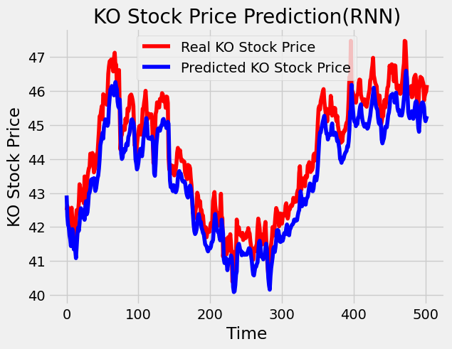
# Evaluating our model
import math
from sklearn.metrics import mean_squared_error
rmse = math.sqrt(mean_squared_error(test_set, predicted_stock_price))
print("The root mean squared error is {}.".format(rmse))
The root mean squared error is 0.7130857635072282.
Now using a LSTM:
# The LSTM architecture
regressor = Sequential()
regressor.add(Input(shape=(X_train.shape[1],1)))
# First LSTM layer with Dropout regularisation
regressor.add(LSTM(units=50))
regressor.add(Dropout(0.3))
regressor.add(Dense(units=1))
regressor.summary()
Model: "sequential_1"
┏━━━━━━━━━━━━━━━━━━━━━━━━━━━━━━━━━┳━━━━━━━━━━━━━━━━━━━━━━━━┳━━━━━━━━━━━━━━━┓
┃ Layer (type)                    ┃ Output Shape           ┃       Param # ┃
┡━━━━━━━━━━━━━━━━━━━━━━━━━━━━━━━━━╇━━━━━━━━━━━━━━━━━━━━━━━━╇━━━━━━━━━━━━━━━┩
│ lstm (LSTM)                     │ (None, 50)             │        10,400 │
├─────────────────────────────────┼────────────────────────┼───────────────┤
│ dropout_1 (Dropout)             │ (None, 50)             │             0 │
├─────────────────────────────────┼────────────────────────┼───────────────┤
│ dense_1 (Dense)                 │ (None, 1)              │            51 │
└─────────────────────────────────┴────────────────────────┴───────────────┘
Total params: 10,451 (40.82 KB)
Trainable params: 10,451 (40.82 KB)
Non-trainable params: 0 (0.00 B)
# Compiling the RNN
regressor.compile(optimizer='adam',loss='mean_squared_error')
# Fitting to the training set
regressor.fit(X_train.reshape(X_train.shape[0],look_back,1),y_train,epochs=50,batch_size=32)
Epoch 1/50
79/79 ━━━━━━━━━━━━━━━━━━━━ 0s 1ms/step - loss: 0.1272
Epoch 2/50
79/79 ━━━━━━━━━━━━━━━━━━━━ 0s 990us/step - loss: 0.0066
Epoch 3/50
79/79 ━━━━━━━━━━━━━━━━━━━━ 0s 1ms/step - loss: 0.0048
Epoch 4/50
79/79 ━━━━━━━━━━━━━━━━━━━━ 0s 1ms/step - loss: 0.0043
Epoch 5/50
79/79 ━━━━━━━━━━━━━━━━━━━━ 0s 1ms/step - loss: 0.0040
Epoch 6/50
79/79 ━━━━━━━━━━━━━━━━━━━━ 0s 991us/step - loss: 0.0038
Epoch 7/50
79/79 ━━━━━━━━━━━━━━━━━━━━ 0s 992us/step - loss: 0.0035
Epoch 8/50
79/79 ━━━━━━━━━━━━━━━━━━━━ 0s 985us/step - loss: 0.0035
Epoch 9/50
79/79 ━━━━━━━━━━━━━━━━━━━━ 0s 984us/step - loss: 0.0037
Epoch 10/50
79/79 ━━━━━━━━━━━━━━━━━━━━ 0s 981us/step - loss: 0.0033
Epoch 11/50
79/79 ━━━━━━━━━━━━━━━━━━━━ 0s 981us/step - loss: 0.0028
Epoch 12/50
79/79 ━━━━━━━━━━━━━━━━━━━━ 0s 1ms/step - loss: 0.0032
Epoch 13/50
79/79 ━━━━━━━━━━━━━━━━━━━━ 0s 1ms/step - loss: 0.0029
Epoch 14/50
79/79 ━━━━━━━━━━━━━━━━━━━━ 0s 1ms/step - loss: 0.0026
Epoch 15/50
79/79 ━━━━━━━━━━━━━━━━━━━━ 0s 986us/step - loss: 0.0029
Epoch 16/50
79/79 ━━━━━━━━━━━━━━━━━━━━ 0s 990us/step - loss: 0.0027
Epoch 17/50
79/79 ━━━━━━━━━━━━━━━━━━━━ 0s 985us/step - loss: 0.0026
Epoch 18/50
79/79 ━━━━━━━━━━━━━━━━━━━━ 0s 985us/step - loss: 0.0027
Epoch 19/50
79/79 ━━━━━━━━━━━━━━━━━━━━ 0s 978us/step - loss: 0.0025
Epoch 20/50
79/79 ━━━━━━━━━━━━━━━━━━━━ 0s 982us/step - loss: 0.0026
Epoch 21/50
79/79 ━━━━━━━━━━━━━━━━━━━━ 0s 981us/step - loss: 0.0024
Epoch 22/50
79/79 ━━━━━━━━━━━━━━━━━━━━ 0s 982us/step - loss: 0.0028
Epoch 23/50
79/79 ━━━━━━━━━━━━━━━━━━━━ 0s 985us/step - loss: 0.0023
Epoch 24/50
79/79 ━━━━━━━━━━━━━━━━━━━━ 0s 983us/step - loss: 0.0023
Epoch 25/50
79/79 ━━━━━━━━━━━━━━━━━━━━ 0s 986us/step - loss: 0.0021
Epoch 26/50
79/79 ━━━━━━━━━━━━━━━━━━━━ 0s 983us/step - loss: 0.0024
Epoch 27/50
79/79 ━━━━━━━━━━━━━━━━━━━━ 0s 984us/step - loss: 0.0020
Epoch 28/50
79/79 ━━━━━━━━━━━━━━━━━━━━ 0s 983us/step - loss: 0.0021
Epoch 29/50
79/79 ━━━━━━━━━━━━━━━━━━━━ 0s 992us/step - loss: 0.0018
Epoch 30/50
79/79 ━━━━━━━━━━━━━━━━━━━━ 0s 1ms/step - loss: 0.0020
Epoch 31/50
79/79 ━━━━━━━━━━━━━━━━━━━━ 0s 1ms/step - loss: 0.0019
Epoch 32/50
79/79 ━━━━━━━━━━━━━━━━━━━━ 0s 991us/step - loss: 0.0019
Epoch 33/50
79/79 ━━━━━━━━━━━━━━━━━━━━ 0s 1ms/step - loss: 0.0017
Epoch 34/50
79/79 ━━━━━━━━━━━━━━━━━━━━ 0s 1ms/step - loss: 0.0018
Epoch 35/50
79/79 ━━━━━━━━━━━━━━━━━━━━ 0s 993us/step - loss: 0.0017
Epoch 36/50
79/79 ━━━━━━━━━━━━━━━━━━━━ 0s 990us/step - loss: 0.0017
Epoch 37/50
79/79 ━━━━━━━━━━━━━━━━━━━━ 0s 987us/step - loss: 0.0015
Epoch 38/50
79/79 ━━━━━━━━━━━━━━━━━━━━ 0s 988us/step - loss: 0.0016
Epoch 39/50
79/79 ━━━━━━━━━━━━━━━━━━━━ 0s 989us/step - loss: 0.0015
Epoch 40/50
79/79 ━━━━━━━━━━━━━━━━━━━━ 0s 1ms/step - loss: 0.0014
Epoch 41/50
79/79 ━━━━━━━━━━━━━━━━━━━━ 0s 1ms/step - loss: 0.0013
Epoch 42/50
79/79 ━━━━━━━━━━━━━━━━━━━━ 0s 1ms/step - loss: 0.0016
Epoch 43/50
79/79 ━━━━━━━━━━━━━━━━━━━━ 0s 1ms/step - loss: 0.0015
Epoch 44/50
79/79 ━━━━━━━━━━━━━━━━━━━━ 0s 1ms/step - loss: 0.0014
Epoch 45/50
79/79 ━━━━━━━━━━━━━━━━━━━━ 0s 1ms/step - loss: 0.0014
Epoch 46/50
79/79 ━━━━━━━━━━━━━━━━━━━━ 0s 1ms/step - loss: 0.0014
Epoch 47/50
79/79 ━━━━━━━━━━━━━━━━━━━━ 0s 1ms/step - loss: 0.0013
Epoch 48/50
79/79 ━━━━━━━━━━━━━━━━━━━━ 0s 1ms/step - loss: 0.0014
Epoch 49/50
79/79 ━━━━━━━━━━━━━━━━━━━━ 0s 1ms/step - loss: 0.0013
Epoch 50/50
79/79 ━━━━━━━━━━━━━━━━━━━━ 0s 1ms/step - loss: 0.0012
<keras.src.callbacks.history.History at 0x32ce9a190>
predicted_stock_price = regressor.predict(X_test)
predicted_stock_price = sc.inverse_transform(predicted_stock_price)
16/16 ━━━━━━━━━━━━━━━━━━━━ 0s 3ms/step
# Visualizing the results
plt.plot(test_set, color='red',label='Real KO Stock Price')
plt.plot(predicted_stock_price, color='blue',label='Predicted KO Stock Price')
plt.title('KO Stock Price Prediction(LSTM)')
plt.xlabel('Time')
plt.ylabel('KO Stock Price')
plt.legend()
plt.show()
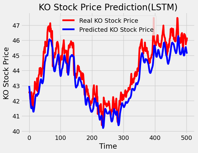
# Evaluating our model
rmse = math.sqrt(mean_squared_error(test_set, predicted_stock_price))
print("The root mean squared error is {}.".format(rmse))
The root mean squared error is 0.8338981916716676.
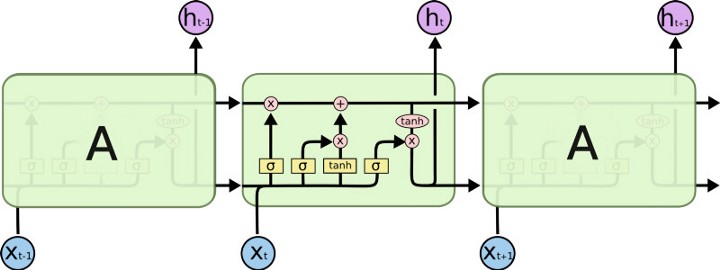
Gated Recurrent Units#
The GRU unit does not have to use a memory unit to control the flow of information like the LSTM unit. It can directly makes use of the all hidden states without any control. GRUs have fewer parameters and thus may train a bit faster or need less data to generalize. But, with large data, the LSTMs with higher expressiveness may lead to better results. Source
Image(filename='local/imgs/lstmandgru.png', width=1200)
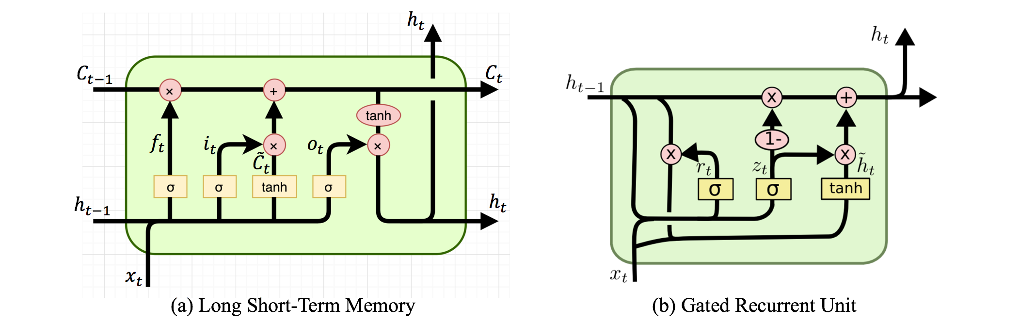
Here \(r\) is a reset gate, and \(z\) is an update gate. Intuitively, the reset gate determines how to combine the new input with the previous memory, and the update gate defines how much of the previous memory to keep around. If set the reset to all 1’s and update gate to all 0’s, it will arrive at the vanilla RNN model.
# The GRU architecture
regressor2 = Sequential()
regressor2.add(Input(shape=(X_train.shape[1],1)))
# First GRU layer with Dropout regularisation
regressor2.add(GRU(units=50))
regressor2.add(Dropout(0.3))
# The output layer
regressor2.add(Dense(units=1))
regressor2.summary()
Model: "sequential_2"
┏━━━━━━━━━━━━━━━━━━━━━━━━━━━━━━━━━┳━━━━━━━━━━━━━━━━━━━━━━━━┳━━━━━━━━━━━━━━━┓
┃ Layer (type)                    ┃ Output Shape           ┃       Param # ┃
┡━━━━━━━━━━━━━━━━━━━━━━━━━━━━━━━━━╇━━━━━━━━━━━━━━━━━━━━━━━━╇━━━━━━━━━━━━━━━┩
│ gru (GRU)                       │ (None, 50)             │         7,950 │
├─────────────────────────────────┼────────────────────────┼───────────────┤
│ dropout_2 (Dropout)             │ (None, 50)             │             0 │
├─────────────────────────────────┼────────────────────────┼───────────────┤
│ dense_2 (Dense)                 │ (None, 1)              │            51 │
└─────────────────────────────────┴────────────────────────┴───────────────┘
Total params: 8,001 (31.25 KB)
Trainable params: 8,001 (31.25 KB)
Non-trainable params: 0 (0.00 B)
# Compiling the RNN
regressor2.compile(optimizer='adam',loss='mean_squared_error')
# Fitting to the training set
regressor2.fit(X_train.reshape(X_train.shape[0],look_back,1),y_train,epochs=50,batch_size=32)
Epoch 1/50
79/79 ━━━━━━━━━━━━━━━━━━━━ 1s 1ms/step - loss: 0.0943
Epoch 2/50
79/79 ━━━━━━━━━━━━━━━━━━━━ 0s 1ms/step - loss: 0.0055
Epoch 3/50
79/79 ━━━━━━━━━━━━━━━━━━━━ 0s 1ms/step - loss: 0.0048
Epoch 4/50
79/79 ━━━━━━━━━━━━━━━━━━━━ 0s 1ms/step - loss: 0.0039
Epoch 5/50
79/79 ━━━━━━━━━━━━━━━━━━━━ 0s 1ms/step - loss: 0.0036
Epoch 6/50
79/79 ━━━━━━━━━━━━━━━━━━━━ 0s 1ms/step - loss: 0.0032
Epoch 7/50
79/79 ━━━━━━━━━━━━━━━━━━━━ 0s 1ms/step - loss: 0.0031
Epoch 8/50
79/79 ━━━━━━━━━━━━━━━━━━━━ 0s 1ms/step - loss: 0.0031
Epoch 9/50
79/79 ━━━━━━━━━━━━━━━━━━━━ 0s 1ms/step - loss: 0.0031
Epoch 10/50
79/79 ━━━━━━━━━━━━━━━━━━━━ 0s 1ms/step - loss: 0.0030
Epoch 11/50
79/79 ━━━━━━━━━━━━━━━━━━━━ 0s 1ms/step - loss: 0.0028
Epoch 12/50
79/79 ━━━━━━━━━━━━━━━━━━━━ 0s 1ms/step - loss: 0.0031
Epoch 13/50
79/79 ━━━━━━━━━━━━━━━━━━━━ 0s 1ms/step - loss: 0.0027
Epoch 14/50
79/79 ━━━━━━━━━━━━━━━━━━━━ 0s 1ms/step - loss: 0.0028
Epoch 15/50
79/79 ━━━━━━━━━━━━━━━━━━━━ 0s 1ms/step - loss: 0.0022
Epoch 16/50
79/79 ━━━━━━━━━━━━━━━━━━━━ 0s 1ms/step - loss: 0.0023
Epoch 17/50
79/79 ━━━━━━━━━━━━━━━━━━━━ 0s 1ms/step - loss: 0.0024
Epoch 18/50
79/79 ━━━━━━━━━━━━━━━━━━━━ 0s 1ms/step - loss: 0.0022
Epoch 19/50
79/79 ━━━━━━━━━━━━━━━━━━━━ 0s 1ms/step - loss: 0.0022
Epoch 20/50
79/79 ━━━━━━━━━━━━━━━━━━━━ 0s 1ms/step - loss: 0.0024
Epoch 21/50
79/79 ━━━━━━━━━━━━━━━━━━━━ 0s 1ms/step - loss: 0.0021
Epoch 22/50
79/79 ━━━━━━━━━━━━━━━━━━━━ 0s 1ms/step - loss: 0.0021
Epoch 23/50
79/79 ━━━━━━━━━━━━━━━━━━━━ 0s 1ms/step - loss: 0.0020
Epoch 24/50
79/79 ━━━━━━━━━━━━━━━━━━━━ 0s 1ms/step - loss: 0.0019
Epoch 25/50
79/79 ━━━━━━━━━━━━━━━━━━━━ 0s 1ms/step - loss: 0.0018
Epoch 26/50
79/79 ━━━━━━━━━━━━━━━━━━━━ 0s 1ms/step - loss: 0.0020
Epoch 27/50
79/79 ━━━━━━━━━━━━━━━━━━━━ 0s 1ms/step - loss: 0.0017
Epoch 28/50
79/79 ━━━━━━━━━━━━━━━━━━━━ 0s 1ms/step - loss: 0.0017
Epoch 29/50
79/79 ━━━━━━━━━━━━━━━━━━━━ 0s 2ms/step - loss: 0.0017
Epoch 30/50
79/79 ━━━━━━━━━━━━━━━━━━━━ 0s 1ms/step - loss: 0.0015
Epoch 31/50
79/79 ━━━━━━━━━━━━━━━━━━━━ 0s 1ms/step - loss: 0.0014
Epoch 32/50
79/79 ━━━━━━━━━━━━━━━━━━━━ 0s 1ms/step - loss: 0.0014
Epoch 33/50
79/79 ━━━━━━━━━━━━━━━━━━━━ 0s 1ms/step - loss: 0.0014
Epoch 34/50
79/79 ━━━━━━━━━━━━━━━━━━━━ 0s 1ms/step - loss: 0.0013
Epoch 35/50
79/79 ━━━━━━━━━━━━━━━━━━━━ 0s 1ms/step - loss: 0.0014
Epoch 36/50
79/79 ━━━━━━━━━━━━━━━━━━━━ 0s 1ms/step - loss: 0.0014
Epoch 37/50
79/79 ━━━━━━━━━━━━━━━━━━━━ 0s 1ms/step - loss: 0.0013
Epoch 38/50
79/79 ━━━━━━━━━━━━━━━━━━━━ 0s 1ms/step - loss: 0.0012
Epoch 39/50
79/79 ━━━━━━━━━━━━━━━━━━━━ 0s 1ms/step - loss: 0.0013
Epoch 40/50
79/79 ━━━━━━━━━━━━━━━━━━━━ 0s 1ms/step - loss: 0.0014
Epoch 41/50
79/79 ━━━━━━━━━━━━━━━━━━━━ 0s 1ms/step - loss: 0.0012
Epoch 42/50
79/79 ━━━━━━━━━━━━━━━━━━━━ 0s 1ms/step - loss: 0.0012
Epoch 43/50
79/79 ━━━━━━━━━━━━━━━━━━━━ 0s 1ms/step - loss: 0.0013
Epoch 44/50
79/79 ━━━━━━━━━━━━━━━━━━━━ 0s 1ms/step - loss: 0.0011
Epoch 45/50
79/79 ━━━━━━━━━━━━━━━━━━━━ 0s 1ms/step - loss: 0.0013
Epoch 46/50
79/79 ━━━━━━━━━━━━━━━━━━━━ 0s 1ms/step - loss: 0.0011
Epoch 47/50
79/79 ━━━━━━━━━━━━━━━━━━━━ 0s 1ms/step - loss: 0.0011
Epoch 48/50
79/79 ━━━━━━━━━━━━━━━━━━━━ 0s 1ms/step - loss: 0.0011
Epoch 49/50
79/79 ━━━━━━━━━━━━━━━━━━━━ 0s 2ms/step - loss: 0.0010
Epoch 50/50
79/79 ━━━━━━━━━━━━━━━━━━━━ 0s 1ms/step - loss: 0.0011
<keras.src.callbacks.history.History at 0x32cf73e20>
Note that the every epoch runs a little bit faster than in the LSTM model.
predicted_stock_price = regressor.predict(X_test)
predicted_stock_price = sc.inverse_transform(predicted_stock_price)
16/16 ━━━━━━━━━━━━━━━━━━━━ 0s 1ms/step
# Visualizing the results
plt.plot(test_set, color='red',label='Real KO Stock Price')
plt.plot(predicted_stock_price, color='blue',label='Predicted KO Stock Price')
plt.title('KO Stock Price Prediction(GRU)')
plt.xlabel('Time')
plt.ylabel('KO Stock Price')
plt.legend()
plt.show()

# Evaluating our model
rmse = math.sqrt(mean_squared_error(test_set, predicted_stock_price))
print("The root mean squared error is {}.".format(rmse))
The root mean squared error is 0.8338981916716676.
Interesting readings:
Understanding LSTM Networks. http://colah.github.io/posts/2015-08-Understanding-LSTMs/