
5.6 Bidirectional RNNs#
!wget -nc --no-cache -O init.py -q https://raw.githubusercontent.com/rramosp/2021.deeplearning/main/content/init.py
import init; init.init(force_download=False);
import tensorflow as tf
import matplotlib.pyplot as plt
import matplotlib.ticker as ticker
from sklearn.model_selection import train_test_split
import unicodedata
import re
import numpy as np
import os
import io
import time
/Users/jdariasl/.cache/uv/archive-v0/mTE5xBvw1heDpxC7T3_--/lib/python3.9/site-packages/urllib3/__init__.py:35: NotOpenSSLWarning: urllib3 v2 only supports OpenSSL 1.1.1+, currently the 'ssl' module is compiled with 'LibreSSL 2.8.3'. See: https://github.com/urllib3/urllib3/issues/3020
  warnings.warn(
from tensorflow.keras.models import Model, Sequential
from tensorflow.keras.layers import GRU, LSTM, Input, Dense, TimeDistributed, Embedding, Activation, RepeatVector, Bidirectional, Concatenate, Dot
from tensorflow.keras.layers import Embedding
from tensorflow.keras.optimizers import Adam
from tensorflow.keras.losses import sparse_categorical_crossentropy
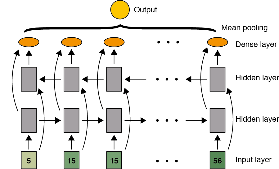
In some problems the information required to make a prediction in one point of a sequence, includes not only pass information but also “future” information, i.e., information before and after of the target point in the sequence. This also implies that such informaction must be available to make the perdictions. For instance, in translation problems usually you need to know an entire sentence beforhand in order to translate it correctly. The bidirectional RNNs are a modification of the standard RNNs that incorporate additional layers which transmit the information from the time \(t+1\) to the time \(t\). The forward and backward layers do not have any conextion among them.
from IPython.display import Image
Image(filename='local/imgs/RNN_arc_3.png', width=1200)
#
Neural Machine Translation#
This example is based on the Machine Translation material included in the Deep Learning Specilization offered by Coursera: https://es.coursera.org/specializations/deep-learning
The following model architecture could be used for a full language translation problem, however it would require hundred of thousands of texts, a big computational power (GPU) and hundreds of hours in order to get a fairly accurate model. Therefore, we are going to use a medium sized datase that includes 118964 sentences in English and Spanish.
# Download the file
path_to_zip = tf.keras.utils.get_file(
    'spa-eng.zip', origin='http://storage.googleapis.com/download.tensorflow.org/data/spa-eng.zip',
    extract=True)

path_to_file = os.path.dirname(path_to_zip)+"/spa-eng_extracted/spa-eng/spa.txt"
# Converts the unicode file to ascii
def unicode_to_ascii(s):
    return ''.join(c for c in unicodedata.normalize('NFD', s)
      if unicodedata.category(c) != 'Mn')


def preprocess_sentence(w):
    w = unicode_to_ascii(w.lower().strip())
    # creating a space between a word and the punctuation following it
    # eg: "he is a boy." => "he is a boy ."
    # Reference:- https://stackoverflow.com/questions/3645931/python-padding-punctuation-with-white-spaces-keeping-punctuation

    w = re.sub(r"([?.!,¿])", r" \1 ", w)
    w = re.sub(r'[" "]+', " ", w)

    # replacing everything with space except (a-z, A-Z, ".", "?", "!", ",")
    w = re.sub(r"[^a-zA-Z?.!,¿]+", " ", w)
    w = w.strip()

    # adding a start and an end token to the sentence
    # so that the model know when to start and stop predicting.
    w = '<start> ' + w + ' <end>'
    return w
en_sentence = u"May I borrow this book?"
sp_sentence = u"¿Puedo tomar prestado este libro?"
print(preprocess_sentence(en_sentence))
print(preprocess_sentence(sp_sentence).encode('utf-8'))
<start> may i borrow this book ? <end>
b'<start> \xc2\xbf puedo tomar prestado este libro ? <end>'
# 1. Remove the accents
# 2. Clean the sentences
# 3. Return word pairs in the format: [ENGLISH, SPANISH]
def create_dataset(path, num_examples):
    lines = io.open(path, encoding='UTF-8').read().strip().split('\n')
    word_pairs = [[preprocess_sentence(w) for w in l.split('\t')]  for l in lines[:num_examples]]
    return zip(*word_pairs)
en, sp = create_dataset(path_to_file, None)
print(en[-1])
print(sp[-1])
<start> if you want to sound like a native speaker , you must be willing to practice saying the same sentence over and over in the same way that banjo players practice the same phrase over and over until they can play it correctly and at the desired tempo . <end>
<start> si quieres sonar como un hablante nativo , debes estar dispuesto a practicar diciendo la misma frase una y otra vez de la misma manera en que un musico de banjo practica el mismo fraseo una y otra vez hasta que lo puedan tocar correctamente y en el tiempo esperado . <end>
len(en),len(sp)
(118964, 118964)
def max_length(tensor):
    return max(len(t) for t in tensor)
Tokenize#
def tokenize(lang):
    lang_tokenizer = tf.keras.preprocessing.text.Tokenizer(
      filters='')
    lang_tokenizer.fit_on_texts(lang)
    tensor = lang_tokenizer.texts_to_sequences(lang)
    tensor = tf.keras.preprocessing.sequence.pad_sequences(tensor,
                                                         padding='post')
    return tensor, lang_tokenizer

def load_dataset(path, num_examples=None):
    # creating cleaned input, output pairs
    targ_lang, inp_lang = create_dataset(path, num_examples)
    input_tensor, inp_lang_tokenizer = tokenize(inp_lang)
    target_tensor, targ_lang_tokenizer = tokenize(targ_lang)

    return input_tensor, target_tensor, inp_lang_tokenizer, targ_lang_tokenizer
Optional#
# Try experimenting with the size of that dataset
num_examples = len(en)#30000
input_tensor, target_tensor, inp_lang, targ_lang = load_dataset(path_to_file, num_examples)

# Calculate max_length of the target tensors
max_length_targ, max_length_inp = max_length(target_tensor), max_length(input_tensor)
# Creating training and validation sets using an 80-20 split
input_tensor_train, input_tensor_val, target_tensor_train, target_tensor_val = train_test_split(input_tensor, target_tensor, test_size=0.2)

# Show length
print(len(input_tensor_train), len(target_tensor_train), len(input_tensor_val), len(target_tensor_val))
95171 95171 23793 23793
len(inp_lang.index_word)
24793
len(targ_lang.index_word)
12933
In order to see the actual Spanish translation, it is necessary to define a function to decode the network’s output.
def convert(lang, tensor):
    for t in tensor:
        if t!=0:
            print ("%d ----> %s" % (t, lang.index_word[t]))
print ("Input Language; index to word mapping")
convert(inp_lang, input_tensor_train[0])
print ()
print ("Target Language; index to word mapping")
convert(targ_lang, target_tensor_train[0])
Input Language; index to word mapping
1 ----> <start>
88 ----> ya
102 ----> habia
1171 ----> tomado
238 ----> cafe
3 ----> .
2 ----> <end>

Target Language; index to word mapping
1 ----> <start>
4 ----> i
71 ----> ve
236 ----> already
60 ----> had
9 ----> a
283 ----> coffee
3 ----> .
2 ----> <end>
input_tensor_train.shape, target_tensor_train.shape
((95171, 53), (95171, 51))
np.expand_dims(input_tensor_train, axis=2).shape
(95171, 53, 1)
Create a tf.data dataset#
For the simplest models, the size of input and output sequences must be equal!
BUFFER_SIZE = len(input_tensor_train)
BATCH_SIZE = 64
steps_per_epoch = len(input_tensor_train)//BATCH_SIZE
embedding_dim = 256
units = 1024
vocab_inp_size = len(inp_lang.word_index)+1
vocab_tar_size = len(targ_lang.word_index)+1

dataset = tf.data.Dataset.from_tensor_slices((np.expand_dims(input_tensor_train, axis=2), np.expand_dims(np.c_[target_tensor_train,np.zeros((target_tensor_train.shape[0],input_tensor_train.shape[1]-target_tensor_train.shape[1]))], axis=2))).shuffle(BUFFER_SIZE)
dataset = dataset.batch(BATCH_SIZE, drop_remainder=True)
example_input_batch, example_target_batch = next(iter(dataset))
example_input_batch.shape, example_target_batch.shape
(TensorShape([64, 53, 1]), TensorShape([64, 53, 1]))
def evaluate1(sentence,model):

    attention_plot = np.zeros((max_length_targ, max_length_inp))
    sentence = preprocess_sentence(sentence)

    inputs = [inp_lang.word_index[i] for i in sentence.split(' ')]
    inputs = tf.keras.preprocessing.sequence.pad_sequences([inputs],
                                                           maxlen=max_length_inp,
                                                           padding='post')
    inputs = tf.convert_to_tensor(inputs)
    result = ''
    out = model.predict(inputs)
    words = out.argmax(axis=-1)
    for t in words[0]:
        if t!=0:
            result += targ_lang.index_word[t] + ' '
    return result
Simple RNN network#
Pay attention to the output format and the loss function.
input_tensor_train.shape[1]
53
def simple_model(input_shape, output_sequence_length, spanish_vocab_size, english_vocab_size):
    learning_rate = 0.001
    input_seq = Input([input_shape[1],1])
    rnn = LSTM(128, return_sequences = True)(input_seq)
    logits = TimeDistributed(Dense(english_vocab_size))(rnn)
    model = Model(input_seq, Activation('softmax')(logits))
    model.compile(loss = 'sparse_categorical_crossentropy',
                 optimizer = Adam(learning_rate))

    return model

# Train the neural network
simple_rnn_model = simple_model(
    input_tensor_train.shape,
    target_tensor_train.shape[1],
    vocab_inp_size,
    vocab_tar_size)
simple_rnn_model.fit(dataset, epochs=50, verbose=1)
simple_rnn_model.summary()
Model: "functional"
┏━━━━━━━━━━━━━━━━━━━━━━━━━━━━━━━━━┳━━━━━━━━━━━━━━━━━━━━━━━━┳━━━━━━━━━━━━━━━┓
┃ Layer (type)                    ┃ Output Shape           ┃       Param # ┃
┡━━━━━━━━━━━━━━━━━━━━━━━━━━━━━━━━━╇━━━━━━━━━━━━━━━━━━━━━━━━╇━━━━━━━━━━━━━━━┩
│ input_layer (InputLayer)        │ (None, 53, 1)          │             0 │
├─────────────────────────────────┼────────────────────────┼───────────────┤
│ lstm (LSTM)                     │ (None, 53, 128)        │        66,560 │
├─────────────────────────────────┼────────────────────────┼───────────────┤
│ time_distributed                │ (None, 53, 12934)      │     1,668,486 │
│ (TimeDistributed)               │                        │               │
├─────────────────────────────────┼────────────────────────┼───────────────┤
│ activation (Activation)         │ (None, 53, 12934)      │             0 │
└─────────────────────────────────┴────────────────────────┴───────────────┘
Total params: 5,205,140 (19.86 MB)
Trainable params: 1,735,046 (6.62 MB)
Non-trainable params: 0 (0.00 B)
Optimizer params: 3,470,094 (13.24 MB)
sentence = u'hace mucho frio en este lugar.'
print(preprocess_sentence(sentence))
result = evaluate1(sentence,simple_rnn_model)
print(result)
<start> hace mucho frio en este lugar . <end>
<start> i ve never in in in . .
sentence = u'esta es mi vida.'
print(preprocess_sentence(sentence))
result = evaluate1(sentence,simple_rnn_model)
print(result)
<start> esta es mi vida . <end>
<start> i is my dog . <end>
Using word2vec#
def embed_model(input_shape, output_sequence_length, spanish_vocab_size, english_vocab_size):
    learning_rate = 0.001
    rnn = LSTM(128, return_sequences=True, activation="relu")

    embedding = Embedding(spanish_vocab_size, 64)
    logits = TimeDistributed(Dense(english_vocab_size, activation="softmax"))

    model = Sequential()
    #em can only be used in first layer --> Keras Documentation
    model.add(Input(shape=(input_shape[1],)))
    model.add(embedding)
    model.add(rnn)
    model.add(logits)
    model.compile(loss='sparse_categorical_crossentropy',
                  optimizer=Adam(learning_rate))

    return model


embeded_model = embed_model(
    input_tensor_train.shape,
    target_tensor_train.shape[1],
    vocab_inp_size,
    vocab_tar_size)

embeded_model.fit(dataset, epochs=50, verbose=1)
1487/1487 ━━━━━━━━━━━━━━━━━━━━ 565s 379ms/step - loss: 2.2396
<keras.src.callbacks.history.History at 0x17f2929a0>
sentence = u'hace mucho frio en este lugar.'
print(preprocess_sentence(sentence))
result = evaluate1(sentence,embeded_model)
print(result)
<start> hace mucho frio en este lugar . <end>
<start> i many cold in in . . <end>
sentence = u'esta es mi vida.'
print(preprocess_sentence(sentence))
result = evaluate1(sentence,embeded_model)
print(result)
<start> esta es mi vida . <end>
<start> this is my life . <end>
Bidirectional RNN#
def bd_model(input_shape, output_sequence_length, spanish_vocab_size, english_vocab_size):

    learning_rate = 0.001
    model = Sequential()
    model.add(Input(shape=(input_shape[1],)))
    model.add(Embedding(spanish_vocab_size, 64))
    model.add(Bidirectional(LSTM(128, return_sequences = True, dropout = 0.1)))
    model.add(TimeDistributed(Dense(english_vocab_size, activation = 'softmax')))
    model.compile(loss = sparse_categorical_crossentropy,
                 optimizer = Adam(learning_rate))
    return model

bidi_model = bd_model(
    input_tensor_train.shape,
    target_tensor_train.shape[1],
    vocab_inp_size,
    vocab_tar_size)

bidi_model.fit(dataset, epochs=50, verbose=1)
Epoch 1/50
1487/1487 [==============================] - 67s 44ms/step - loss: 1.5199
Epoch 2/50
1487/1487 [==============================] - 65s 44ms/step - loss: 0.7412
Epoch 3/50
1487/1487 [==============================] - 65s 43ms/step - loss: 0.6230
Epoch 4/50
1487/1487 [==============================] - 65s 44ms/step - loss: 0.5487
Epoch 5/50
1487/1487 [==============================] - 65s 44ms/step - loss: 0.4892
Epoch 6/50
1487/1487 [==============================] - 65s 44ms/step - loss: 0.4481
Epoch 7/50
1487/1487 [==============================] - 65s 44ms/step - loss: 0.4140
Epoch 8/50
1487/1487 [==============================] - 65s 44ms/step - loss: 0.3863
Epoch 9/50
1487/1487 [==============================] - 65s 44ms/step - loss: 0.3629
Epoch 10/50
1487/1487 [==============================] - 65s 44ms/step - loss: 0.3422
Epoch 11/50
1487/1487 [==============================] - 65s 44ms/step - loss: 0.3274
Epoch 12/50
1487/1487 [==============================] - 65s 44ms/step - loss: 0.3117
Epoch 13/50
1487/1487 [==============================] - 65s 43ms/step - loss: 0.2999
Epoch 14/50
1487/1487 [==============================] - 65s 44ms/step - loss: 0.2901
Epoch 15/50
1487/1487 [==============================] - 65s 44ms/step - loss: 0.2811
Epoch 16/50
1487/1487 [==============================] - 65s 44ms/step - loss: 0.2730
Epoch 17/50
1487/1487 [==============================] - 65s 44ms/step - loss: 0.2665
Epoch 18/50
1487/1487 [==============================] - 65s 44ms/step - loss: 0.2599
Epoch 19/50
1487/1487 [==============================] - 65s 44ms/step - loss: 0.2557
Epoch 20/50
1487/1487 [==============================] - 65s 44ms/step - loss: 0.2493
Epoch 21/50
1487/1487 [==============================] - 65s 44ms/step - loss: 0.2458
Epoch 22/50
1487/1487 [==============================] - 65s 43ms/step - loss: 0.2396
Epoch 23/50
1487/1487 [==============================] - 65s 44ms/step - loss: 0.2357
Epoch 24/50
1487/1487 [==============================] - 65s 44ms/step - loss: 0.2335
Epoch 25/50
1487/1487 [==============================] - 65s 43ms/step - loss: 0.2286
Epoch 26/50
1487/1487 [==============================] - 65s 43ms/step - loss: 0.2256
Epoch 27/50
1487/1487 [==============================] - 65s 44ms/step - loss: 0.2230
Epoch 28/50
1487/1487 [==============================] - 65s 44ms/step - loss: 0.2189
Epoch 29/50
1487/1487 [==============================] - 65s 44ms/step - loss: 0.2168
Epoch 30/50
1487/1487 [==============================] - 64s 43ms/step - loss: 0.2144
Epoch 31/50
1487/1487 [==============================] - 64s 43ms/step - loss: 0.2108
Epoch 32/50
1487/1487 [==============================] - 65s 43ms/step - loss: 0.2097
Epoch 33/50
1487/1487 [==============================] - 65s 44ms/step - loss: 0.2074
Epoch 34/50
1487/1487 [==============================] - 65s 43ms/step - loss: 0.2054
Epoch 35/50
1487/1487 [==============================] - 65s 43ms/step - loss: 0.2029
Epoch 36/50
1487/1487 [==============================] - 64s 43ms/step - loss: 0.2003
Epoch 37/50
1487/1487 [==============================] - 65s 43ms/step - loss: 0.1982
Epoch 38/50
1487/1487 [==============================] - 64s 43ms/step - loss: 0.1988
Epoch 39/50
1487/1487 [==============================] - 65s 43ms/step - loss: 0.1975
Epoch 40/50
1487/1487 [==============================] - 64s 43ms/step - loss: 0.1945
Epoch 41/50
1487/1487 [==============================] - 65s 43ms/step - loss: 0.1936
Epoch 42/50
1487/1487 [==============================] - 64s 43ms/step - loss: 0.1934
Epoch 43/50
1487/1487 [==============================] - 64s 43ms/step - loss: 0.1913
Epoch 44/50
1487/1487 [==============================] - 64s 43ms/step - loss: 0.1890
Epoch 45/50
1487/1487 [==============================] - 64s 43ms/step - loss: 0.1880
Epoch 46/50
1487/1487 [==============================] - 64s 43ms/step - loss: 0.1882
Epoch 47/50
1487/1487 [==============================] - 64s 43ms/step - loss: 0.1855
Epoch 48/50
1487/1487 [==============================] - 64s 43ms/step - loss: 0.1848
Epoch 49/50
1487/1487 [==============================] - 64s 43ms/step - loss: 0.1843
Epoch 50/50
1487/1487 [==============================] - 64s 43ms/step - loss: 0.1821
<tensorflow.python.keras.callbacks.History at 0x7f08eb5d0cd0>
bidi_model.summary()
Model: "sequential_1"
_________________________________________________________________
Layer (type)                 Output Shape              Param #
=================================================================
embedding_1 (Embedding)      (None, 53, 64)            1586816
_________________________________________________________________
bidirectional (Bidirectional (None, 53, 256)           197632
_________________________________________________________________
time_distributed_2 (TimeDist (None, 53, 12934)         3324038
=================================================================
Total params: 5,108,486
Trainable params: 5,108,486
Non-trainable params: 0
_________________________________________________________________
sentence = u'hace mucho frio en este lugar.'
print(preprocess_sentence(sentence))
result = evaluate1(sentence,bidi_model)
print(result)
<start> hace mucho frio en este lugar . <end>
<start> it s is cold of this place . <end>
sentence = u'esta es mi vida.'
print(preprocess_sentence(sentence))
result = evaluate1(sentence,bidi_model)
print(result)
<start> esta es mi vida . <end>
<start> this is my life . <end>
Encoder-decoder#
from IPython.display import Image
Image(filename='local/imgs/EDA.png', width=1200)
#
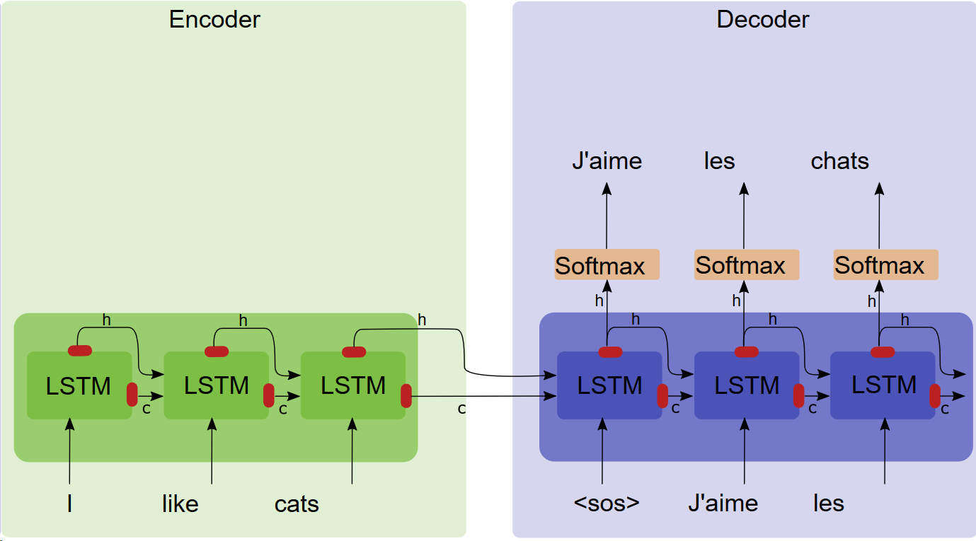
Image taken from: https://towardsdatascience.com/light-on-math-ml-attention-with-keras-dc8dbc1fad39
This model is able to deal with input and output sequences of different length!
BUFFER_SIZE = len(input_tensor_train)
BATCH_SIZE = 64
steps_per_epoch = len(input_tensor_train)//BATCH_SIZE
embedding_dim = 256
units = 1024
vocab_inp_size = len(inp_lang.word_index)+1
vocab_tar_size = len(targ_lang.word_index)+1

dataset = tf.data.Dataset.from_tensor_slices((input_tensor_train, target_tensor_train)).shuffle(BUFFER_SIZE)
dataset = dataset.batch(BATCH_SIZE, drop_remainder=True)
example_input_batch, example_target_batch = next(iter(dataset))
example_input_batch.shape, example_target_batch.shape
(TensorShape([64, 53]), TensorShape([64, 51]))
def encdec_model(input_shape, output_sequence_length, english_vocab_size, spanish_vocab_size):

    learning_rate = 0.001
    model = Sequential()
    model.add(Input(shape=(input_shape[1],)))
    model.add(Embedding(input_dim=english_vocab_size, output_dim=64))
    model.add(Bidirectional(LSTM(256, return_sequences = False)))
    model.add(RepeatVector(output_sequence_length))
    model.add(LSTM(256, return_sequences = True))
    model.add(TimeDistributed(Dense(spanish_vocab_size, activation = 'softmax')))

    model.compile(loss = 'sparse_categorical_crossentropy',
                 optimizer = Adam(learning_rate))
    return model


encodeco_model = encdec_model(
    input_tensor_train.shape,
    target_tensor_train.shape[1],
    vocab_inp_size,
    vocab_tar_size)

encodeco_model.fit(dataset, epochs=50, verbose=1)
Epoch 1/50
1487/1487 [==============================] - 78s 51ms/step - loss: 1.5090
Epoch 2/50
1487/1487 [==============================] - 75s 50ms/step - loss: 0.9854
Epoch 3/50
1487/1487 [==============================] - 72s 49ms/step - loss: 0.9288
Epoch 4/50
1487/1487 [==============================] - 71s 48ms/step - loss: 0.8489
Epoch 5/50
1487/1487 [==============================] - 71s 48ms/step - loss: 0.7870
Epoch 6/50
1487/1487 [==============================] - 71s 48ms/step - loss: 0.7361
Epoch 7/50
1487/1487 [==============================] - 71s 48ms/step - loss: 0.6871
Epoch 8/50
1487/1487 [==============================] - 71s 48ms/step - loss: 0.6398
Epoch 9/50
1487/1487 [==============================] - 71s 48ms/step - loss: 0.5965
Epoch 10/50
1487/1487 [==============================] - 68s 46ms/step - loss: 0.5552
Epoch 11/50
1487/1487 [==============================] - 69s 47ms/step - loss: 0.5217
Epoch 12/50
1487/1487 [==============================] - 72s 48ms/step - loss: 0.4909
Epoch 13/50
1487/1487 [==============================] - 71s 48ms/step - loss: 0.4607
Epoch 14/50
1487/1487 [==============================] - 71s 48ms/step - loss: 0.4374
Epoch 15/50
1487/1487 [==============================] - 72s 48ms/step - loss: 0.4122
Epoch 16/50
1487/1487 [==============================] - 70s 47ms/step - loss: 0.3900
Epoch 17/50
1487/1487 [==============================] - 71s 48ms/step - loss: 0.3716
Epoch 18/50
1487/1487 [==============================] - 71s 48ms/step - loss: 0.3542
Epoch 19/50
1487/1487 [==============================] - 71s 47ms/step - loss: 0.3386
Epoch 20/50
1487/1487 [==============================] - 71s 47ms/step - loss: 0.3265
Epoch 21/50
1487/1487 [==============================] - 69s 46ms/step - loss: 0.3133
Epoch 22/50
1487/1487 [==============================] - 68s 46ms/step - loss: 0.3032
Epoch 23/50
1487/1487 [==============================] - 68s 46ms/step - loss: 0.2893
Epoch 24/50
1487/1487 [==============================] - 68s 45ms/step - loss: 0.2798
Epoch 25/50
1487/1487 [==============================] - 68s 45ms/step - loss: 0.2705
Epoch 26/50
1487/1487 [==============================] - 68s 45ms/step - loss: 0.2635
Epoch 27/50
1487/1487 [==============================] - 68s 46ms/step - loss: 0.2529
Epoch 28/50
1487/1487 [==============================] - 68s 46ms/step - loss: 0.2468
Epoch 29/50
1487/1487 [==============================] - 71s 48ms/step - loss: 0.2389
Epoch 30/50
1487/1487 [==============================] - 70s 47ms/step - loss: 0.2343
Epoch 31/50
1487/1487 [==============================] - 71s 48ms/step - loss: 0.2282
Epoch 32/50
1487/1487 [==============================] - 73s 49ms/step - loss: 0.2216
Epoch 33/50
1487/1487 [==============================] - 73s 49ms/step - loss: 0.2154
Epoch 34/50
1487/1487 [==============================] - 76s 51ms/step - loss: 0.2085
Epoch 35/50
1487/1487 [==============================] - 75s 50ms/step - loss: 0.2047
Epoch 36/50
1487/1487 [==============================] - 64s 43ms/step - loss: 0.1993
Epoch 37/50
1487/1487 [==============================] - 66s 44ms/step - loss: 0.1968
Epoch 38/50
1487/1487 [==============================] - 68s 46ms/step - loss: 0.1902
Epoch 39/50
1487/1487 [==============================] - 70s 47ms/step - loss: 0.1858
Epoch 40/50
1487/1487 [==============================] - 70s 47ms/step - loss: 0.1813
Epoch 41/50
1487/1487 [==============================] - 69s 46ms/step - loss: 0.1783
Epoch 42/50
1487/1487 [==============================] - 66s 44ms/step - loss: 0.1739
Epoch 43/50
1487/1487 [==============================] - 62s 42ms/step - loss: 0.1682
Epoch 44/50
1487/1487 [==============================] - 62s 42ms/step - loss: 0.1661
Epoch 45/50
1487/1487 [==============================] - 62s 42ms/step - loss: 0.1622
Epoch 46/50
1487/1487 [==============================] - 62s 42ms/step - loss: 0.1596
Epoch 47/50
1487/1487 [==============================] - 62s 42ms/step - loss: 0.1572
Epoch 48/50
1487/1487 [==============================] - 62s 42ms/step - loss: 0.1535
Epoch 49/50
1487/1487 [==============================] - 62s 42ms/step - loss: 0.1501
Epoch 50/50
1487/1487 [==============================] - 62s 42ms/step - loss: 0.1486
<tensorflow.python.keras.callbacks.History at 0x7f09d45b0390>
encodeco_model.summary()
Model: "sequential_2"
_________________________________________________________________
Layer (type)                 Output Shape              Param #
=================================================================
embedding_2 (Embedding)      (None, 53, 64)            1586816
_________________________________________________________________
bidirectional_1 (Bidirection (None, 512)               657408
_________________________________________________________________
repeat_vector (RepeatVector) (None, 51, 512)           0
_________________________________________________________________
lstm_4 (LSTM)                (None, 51, 256)           787456
_________________________________________________________________
time_distributed_3 (TimeDist (None, 51, 12934)         3324038
=================================================================
Total params: 6,355,718
Trainable params: 6,355,718
Non-trainable params: 0
_________________________________________________________________
sentence = u'hace mucho frio en este lugar.'
print(preprocess_sentence(sentence))
result = evaluate1(sentence,encodeco_model)
print(result)
<start> hace mucho frio en este lugar . <end>
<start> it artist is cold this this this . <end>
sentence = u'esta es mi vida.'
print(preprocess_sentence(sentence))
result = evaluate1(sentence,encodeco_model)
print(result)
<start> esta es mi vida . <end>
<start> this is my life . <end>
Neural machine translation with attention#
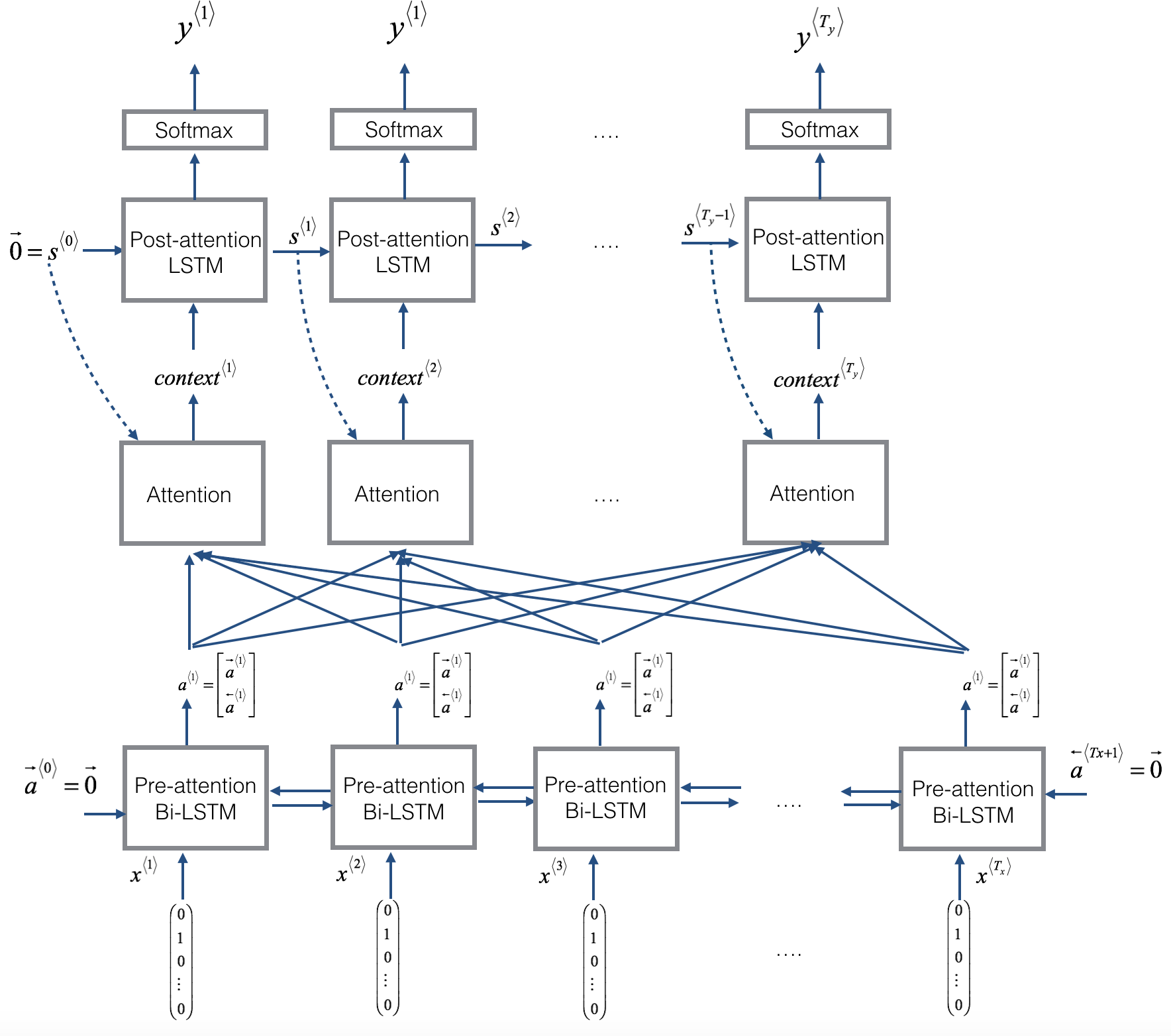
One of the problems of the previous model is the fact that the model has to memorize the entire sentence before start to translate it. The attention model introduces and additional layer that weight the contribution of the first bidirectional RNN layer’s outputs to be feed into the last recurrent layer.
Dzmitry Bahdanau, Kyunghyun Cho, Yoshua Bengio , Neural Machine Translation by Jointly Learning to Align and Translate. https://arxiv.org/abs/1409.0473
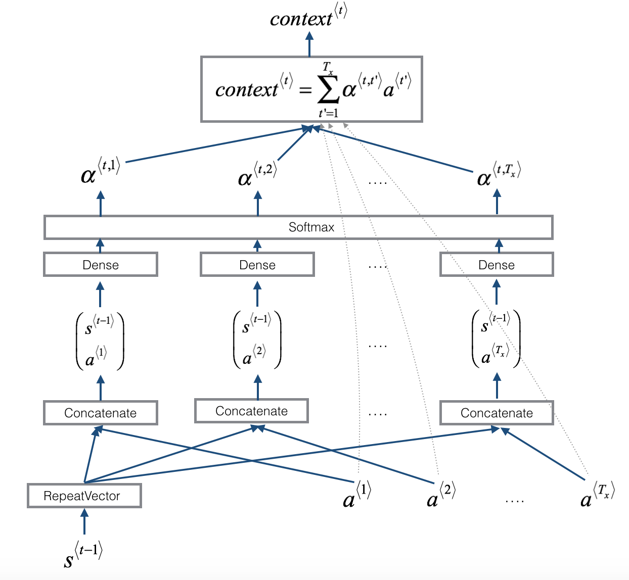
Image(filename='local/imgs/attn_model.png', width=800)
Image(filename='local/imgs/attn_mechanism.png', width=800)
In the following you can see the implementation of the attention model. Each component of the model is defined independently: Encoder, BahdanauAttention and Decoder. During training, the Encoder is called one time, and the decoder is called recursively once per word in the target language.
Example taken from: link
class Encoder(tf.keras.Model):
    def __init__(self, vocab_size, embedding_dim, enc_units, batch_sz):
        super(Encoder, self).__init__()
        self.batch_sz = batch_sz
        self.enc_units = enc_units
        self.embedding = tf.keras.layers.Embedding(vocab_size, embedding_dim)
        self.gru = tf.keras.layers.GRU(self.enc_units,
                                       return_sequences=True,
                                       return_state=True,
                                       recurrent_initializer='glorot_uniform')

    def call(self, x, hidden):
        x = self.embedding(x)
        output, state = self.gru(x, initial_state = hidden)
        return output, state

    def initialize_hidden_state(self):
        return tf.zeros((self.batch_sz, self.enc_units))
encoder = Encoder(vocab_inp_size, embedding_dim, units, BATCH_SIZE)

# sample input
sample_hidden = encoder.initialize_hidden_state()
sample_output, sample_hidden = encoder(example_input_batch, sample_hidden)
print ('Encoder output shape: (batch size, sequence length, units) {}'.format(sample_output.shape))
print ('Encoder Hidden state shape: (batch size, units) {}'.format(sample_hidden.shape))
Encoder output shape: (batch size, sequence length, units) (64, 53, 1024)
Encoder Hidden state shape: (batch size, units) (64, 1024)
class BahdanauAttention(tf.keras.layers.Layer):
    def __init__(self, units):
        super(BahdanauAttention, self).__init__()
        self.W1 = tf.keras.layers.Dense(units)
        self.W2 = tf.keras.layers.Dense(units)
        self.V = tf.keras.layers.Dense(1)

    def call(self, query, values):
        # query hidden state shape == (batch_size, hidden size)
        # query_with_time_axis shape == (batch_size, 1, hidden size)
        # values shape == (batch_size, max_len, hidden size)
        # we are doing this to broadcast addition along the time axis to calculate the score
        query_with_time_axis = tf.expand_dims(query, 1)

        # score shape == (batch_size, max_length, 1)
        # we get 1 at the last axis because we are applying score to self.V
        # the shape of the tensor before applying self.V is (batch_size, max_length, units)
        score = self.V(tf.nn.tanh(self.W1(query_with_time_axis) + self.W2(values)))

        # attention_weights shape == (batch_size, max_length, 1)
        attention_weights = tf.nn.softmax(score, axis=1)

        # context_vector shape after sum == (batch_size, hidden_size)
        context_vector = attention_weights * values
        context_vector = tf.reduce_sum(context_vector, axis=1)

        return context_vector, attention_weights
attention_layer = BahdanauAttention(10)
attention_result, attention_weights = attention_layer(sample_hidden, sample_output)

print("Attention result shape: (batch size, units) {}".format(attention_result.shape))
print("Attention weights shape: (batch_size, sequence_length, 1) {}".format(attention_weights.shape))
Attention result shape: (batch size, units) (64, 1024)
Attention weights shape: (batch_size, sequence_length, 1) (64, 53, 1)
class Decoder(tf.keras.Model):
    def __init__(self, vocab_size, embedding_dim, dec_units, batch_sz):
        super(Decoder, self).__init__()
        self.batch_sz = batch_sz
        self.dec_units = dec_units
        self.embedding = tf.keras.layers.Embedding(vocab_size, embedding_dim)
        self.gru = tf.keras.layers.GRU(self.dec_units,
                                       return_sequences=True,
                                       return_state=True,
                                       recurrent_initializer='glorot_uniform')
        self.fc = tf.keras.layers.Dense(vocab_size)

        # used for attention
        self.attention = BahdanauAttention(self.dec_units)


    def call(self, x, hidden, enc_output):
        # enc_output shape == (batch_size, max_length, hidden_size)
        context_vector, attention_weights = self.attention(hidden, enc_output)


        # x shape after passing through embedding == (batch_size, 1, embedding_dim)
        x = self.embedding(x)

        # x shape after concatenation == (batch_size, 1, embedding_dim + hidden_size
        x = tf.concat([tf.expand_dims(context_vector, 1), x], axis=-1)

        # passing the concatenated vector to the GRU
        output, state = self.gru(x)

        # output shape == (batch_size * 1, hidden_size)
        output = tf.reshape(output, (-1, output.shape[2]))

        # output shape == (batch_size, vocab)
        x = self.fc(output)

        return x, state, attention_weights
decoder = Decoder(vocab_tar_size, embedding_dim, units, BATCH_SIZE)

sample_decoder_output, _, _ = decoder(tf.random.uniform((BATCH_SIZE, 1)),
                                      sample_hidden, sample_output)

print ('Decoder output shape: (batch_size, vocab size) {}'.format(sample_decoder_output.shape))
Decoder output shape: (batch_size, vocab size) (64, 12934)
optimizer = tf.keras.optimizers.Adam()
loss_object = tf.keras.losses.SparseCategoricalCrossentropy(
    from_logits=True, reduction='none')

def loss_function(real, pred):

    mask = tf.math.logical_not(tf.math.equal(real, 0))
    loss_ = loss_object(real, pred)

    mask = tf.cast(mask, dtype=loss_.dtype)
    loss_ *= mask

    return tf.reduce_mean(loss_)
checkpoint_dir = './training_checkpoints'
checkpoint_prefix = os.path.join(checkpoint_dir, "ckpt")
checkpoint = tf.train.Checkpoint(optimizer=optimizer,
                                 encoder=encoder,
                                 decoder=decoder)
@tf.function
def train_step(inp, targ, enc_hidden):
    loss = 0

    with tf.GradientTape() as tape:
        enc_output, enc_hidden = encoder(inp, enc_hidden)
        dec_hidden = enc_hidden

        dec_input = tf.expand_dims([targ_lang.word_index['<start>']] * BATCH_SIZE, 1)

        # Teacher forcing - feeding the target as the next input
        for t in range(1, targ.shape[1]):
            # passing enc_output to the decoder
            predictions, dec_hidden, _ = decoder(dec_input, dec_hidden, enc_output)
            loss += loss_function(targ[:, t], predictions)
            # using teacher forcing
            dec_input = tf.expand_dims(targ[:, t], 1)

    batch_loss = (loss / int(targ.shape[1]))
    variables = encoder.trainable_variables + decoder.trainable_variables
    gradients = tape.gradient(loss, variables)
    optimizer.apply_gradients(zip(gradients, variables))

    return batch_loss
EPOCHS = 10

for epoch in range(EPOCHS):
    start = time.time()

    enc_hidden = encoder.initialize_hidden_state()
    total_loss = 0

    for (batch, (inp, targ)) in enumerate(dataset.take(steps_per_epoch)):
        batch_loss = train_step(inp, targ, enc_hidden)
        total_loss += batch_loss

        if batch % 100 == 0:
            print('Epoch {} Batch {} Loss {:.4f}'.format(epoch + 1,
                                                         batch,
                                                         batch_loss.numpy()))
    # saving (checkpoint) the model every 2 epochs
    if (epoch + 1) % 2 == 0:
        checkpoint.save(file_prefix = checkpoint_prefix)
    print('Epoch {} Loss {:.4f}'.format(epoch + 1,
                                        total_loss / steps_per_epoch))
    print('Time taken for 1 epoch {} sec\n'.format(time.time() - start))
Epoch 1 Batch 0 Loss 1.7346
Epoch 1 Batch 100 Loss 0.8601
Epoch 1 Batch 200 Loss 0.7552
Epoch 1 Batch 300 Loss 0.8281
Epoch 1 Batch 400 Loss 0.6538
Epoch 1 Batch 500 Loss 0.6904
Epoch 1 Batch 600 Loss 0.5495
Epoch 1 Batch 700 Loss 0.5438
Epoch 1 Batch 800 Loss 0.5842
Epoch 1 Batch 900 Loss 0.5163
Epoch 1 Batch 1000 Loss 0.5993
Epoch 1 Batch 1100 Loss 0.4308
Epoch 1 Batch 1200 Loss 0.4373
Epoch 1 Batch 1300 Loss 0.4032
Epoch 1 Batch 1400 Loss 0.3693
Epoch 1 Loss 0.6021
Time taken for 1 epoch 476.49583768844604 sec

Epoch 2 Batch 0 Loss 0.3239
Epoch 2 Batch 100 Loss 0.2871
Epoch 2 Batch 200 Loss 0.3192
Epoch 2 Batch 300 Loss 0.3301
Epoch 2 Batch 400 Loss 0.2794
Epoch 2 Batch 500 Loss 0.2810
Epoch 2 Batch 600 Loss 0.2682
Epoch 2 Batch 700 Loss 0.2927
Epoch 2 Batch 800 Loss 0.2909
Epoch 2 Batch 900 Loss 0.2823
Epoch 2 Batch 1000 Loss 0.2315
Epoch 2 Batch 1100 Loss 0.2200
Epoch 2 Batch 1200 Loss 0.2360
Epoch 2 Batch 1300 Loss 0.3076
Epoch 2 Batch 1400 Loss 0.2552
Epoch 2 Loss 0.2948
Time taken for 1 epoch 443.41202902793884 sec

Epoch 3 Batch 0 Loss 0.2245
Epoch 3 Batch 100 Loss 0.1588
Epoch 3 Batch 200 Loss 0.2158
Epoch 3 Batch 300 Loss 0.1791
Epoch 3 Batch 400 Loss 0.2155
Epoch 3 Batch 500 Loss 0.1926
Epoch 3 Batch 600 Loss 0.1355
Epoch 3 Batch 700 Loss 0.2063
Epoch 3 Batch 800 Loss 0.1654
Epoch 3 Batch 900 Loss 0.2098
Epoch 3 Batch 1000 Loss 0.1720
Epoch 3 Batch 1100 Loss 0.1925
Epoch 3 Batch 1200 Loss 0.2301
Epoch 3 Batch 1300 Loss 0.1985
Epoch 3 Batch 1400 Loss 0.1597
Epoch 3 Loss 0.1901
Time taken for 1 epoch 442.3017530441284 sec

Epoch 4 Batch 0 Loss 0.1536
Epoch 4 Batch 100 Loss 0.1502
Epoch 4 Batch 200 Loss 0.1614
Epoch 4 Batch 300 Loss 0.1211
Epoch 4 Batch 400 Loss 0.1329
Epoch 4 Batch 500 Loss 0.1426
Epoch 4 Batch 600 Loss 0.1953
Epoch 4 Batch 700 Loss 0.1445
Epoch 4 Batch 800 Loss 0.1316
Epoch 4 Batch 900 Loss 0.1397
Epoch 4 Batch 1000 Loss 0.1414
Epoch 4 Batch 1100 Loss 0.1160
Epoch 4 Batch 1200 Loss 0.1254
Epoch 4 Batch 1300 Loss 0.1146
Epoch 4 Batch 1400 Loss 0.1300
Epoch 4 Loss 0.1361
Time taken for 1 epoch 447.2612314224243 sec

Epoch 5 Batch 0 Loss 0.0945
Epoch 5 Batch 100 Loss 0.0898
Epoch 5 Batch 200 Loss 0.0932
Epoch 5 Batch 300 Loss 0.0998
Epoch 5 Batch 400 Loss 0.1076
Epoch 5 Batch 500 Loss 0.0898
Epoch 5 Batch 600 Loss 0.0908
Epoch 5 Batch 700 Loss 0.1156
Epoch 5 Batch 800 Loss 0.1284
Epoch 5 Batch 900 Loss 0.1172
Epoch 5 Batch 1000 Loss 0.1147
Epoch 5 Batch 1100 Loss 0.1418
Epoch 5 Batch 1200 Loss 0.1449
Epoch 5 Batch 1300 Loss 0.1080
Epoch 5 Batch 1400 Loss 0.1143
Epoch 5 Loss 0.1017
Time taken for 1 epoch 443.46099615097046 sec

Epoch 6 Batch 0 Loss 0.0676
Epoch 6 Batch 100 Loss 0.0590
Epoch 6 Batch 200 Loss 0.0687
Epoch 6 Batch 300 Loss 0.0728
Epoch 6 Batch 400 Loss 0.0694
Epoch 6 Batch 500 Loss 0.0802
Epoch 6 Batch 600 Loss 0.0742
Epoch 6 Batch 700 Loss 0.0848
Epoch 6 Batch 800 Loss 0.0692
Epoch 6 Batch 900 Loss 0.0680
Epoch 6 Batch 1000 Loss 0.1037
Epoch 6 Batch 1100 Loss 0.0854
Epoch 6 Batch 1200 Loss 0.0880
Epoch 6 Batch 1300 Loss 0.0917
Epoch 6 Batch 1400 Loss 0.0787
Epoch 6 Loss 0.0801
Time taken for 1 epoch 451.2902102470398 sec

Epoch 7 Batch 0 Loss 0.0555
Epoch 7 Batch 100 Loss 0.0473
Epoch 7 Batch 200 Loss 0.0644
Epoch 7 Batch 300 Loss 0.0929
Epoch 7 Batch 400 Loss 0.0679
Epoch 7 Batch 500 Loss 0.0831
Epoch 7 Batch 600 Loss 0.0495
Epoch 7 Batch 700 Loss 0.0898
Epoch 7 Batch 800 Loss 0.0817
Epoch 7 Batch 900 Loss 0.0727
Epoch 7 Batch 1000 Loss 0.0696
Epoch 7 Batch 1100 Loss 0.0620
Epoch 7 Batch 1200 Loss 0.0658
Epoch 7 Batch 1300 Loss 0.0600
Epoch 7 Batch 1400 Loss 0.0772
Epoch 7 Loss 0.0663
Time taken for 1 epoch 444.74028038978577 sec

Epoch 8 Batch 0 Loss 0.0424
Epoch 8 Batch 100 Loss 0.0421
Epoch 8 Batch 200 Loss 0.0640
Epoch 8 Batch 300 Loss 0.0477
Epoch 8 Batch 400 Loss 0.0493
Epoch 8 Batch 500 Loss 0.0531
Epoch 8 Batch 600 Loss 0.0471
Epoch 8 Batch 700 Loss 0.0569
Epoch 8 Batch 800 Loss 0.0582
Epoch 8 Batch 900 Loss 0.0611
Epoch 8 Batch 1000 Loss 0.0451
Epoch 8 Batch 1100 Loss 0.0607
Epoch 8 Batch 1200 Loss 0.0544
Epoch 8 Batch 1300 Loss 0.0822
Epoch 8 Batch 1400 Loss 0.0597
Epoch 8 Loss 0.0512
Time taken for 1 epoch 451.4748868942261 sec

Epoch 9 Batch 0 Loss 0.0312
Epoch 9 Batch 100 Loss 0.0306
Epoch 9 Batch 200 Loss 0.0266
Epoch 9 Batch 300 Loss 0.0255
Epoch 9 Batch 400 Loss 0.0425
Epoch 9 Batch 500 Loss 0.0346
Epoch 9 Batch 600 Loss 0.0438
Epoch 9 Batch 700 Loss 0.0360
Epoch 9 Batch 800 Loss 0.0434
Epoch 9 Batch 900 Loss 0.0495
Epoch 9 Batch 1000 Loss 0.0403
Epoch 9 Batch 1100 Loss 0.0514
Epoch 9 Batch 1200 Loss 0.0354
Epoch 9 Batch 1300 Loss 0.0545
Epoch 9 Batch 1400 Loss 0.0485
Epoch 9 Loss 0.0447
Time taken for 1 epoch 475.8938076496124 sec

Epoch 10 Batch 0 Loss 0.0410
Epoch 10 Batch 100 Loss 0.0339
Epoch 10 Batch 200 Loss 0.0308
Epoch 10 Batch 300 Loss 0.0359
Epoch 10 Batch 400 Loss 0.0359
Epoch 10 Batch 500 Loss 0.0458
Epoch 10 Batch 600 Loss 0.0357
Epoch 10 Batch 700 Loss 0.0306
Epoch 10 Batch 800 Loss 0.0564
Epoch 10 Batch 900 Loss 0.0458
Epoch 10 Batch 1000 Loss 0.0346
Epoch 10 Batch 1100 Loss 0.0481
Epoch 10 Batch 1200 Loss 0.0486
Epoch 10 Batch 1300 Loss 0.0386
Epoch 10 Batch 1400 Loss 0.0599
Epoch 10 Loss 0.0396
Time taken for 1 epoch 481.80025815963745 sec
def evaluate(sentence):

    attention_plot = np.zeros((max_length_targ, max_length_inp))
    sentence = preprocess_sentence(sentence)

    inputs = [inp_lang.word_index[i] for i in sentence.split(' ')]
    inputs = tf.keras.preprocessing.sequence.pad_sequences([inputs],
                                                           maxlen=max_length_inp,
                                                           padding='post')
    inputs = tf.convert_to_tensor(inputs)
    result = ''

    hidden = [tf.zeros((1, units))]
    enc_out, enc_hidden = encoder(inputs, hidden)

    dec_hidden = enc_hidden
    dec_input = tf.expand_dims([targ_lang.word_index['<start>']], 0)

    for t in range(max_length_targ):
        predictions, dec_hidden, attention_weights = decoder(dec_input,
                                                             dec_hidden,
                                                             enc_out)

        # storing the attention weights to plot later on
        attention_weights = tf.reshape(attention_weights, (-1, ))
        attention_plot[t] = attention_weights.numpy()

        predicted_id = tf.argmax(predictions[0]).numpy()
        result += targ_lang.index_word[predicted_id] + ' '

        if targ_lang.index_word[predicted_id] == '<end>':
            return result, sentence, attention_plot

        # the predicted ID is fed back into the model
        dec_input = tf.expand_dims([predicted_id], 0)
    return result, sentence, attention_plot
# function for plotting the attention weights
def plot_attention(attention, sentence, predicted_sentence):
    fig = plt.figure(figsize=(10,10))
    ax = fig.add_subplot(1, 1, 1)
    ax.matshow(attention, cmap='viridis')

    fontdict = {'fontsize': 14}
    ax.set_xticklabels([''] + sentence, fontdict=fontdict, rotation=90)
    ax.set_yticklabels([''] + predicted_sentence, fontdict=fontdict)

    ax.xaxis.set_major_locator(ticker.MultipleLocator(1))
    ax.yaxis.set_major_locator(ticker.MultipleLocator(1))

    plt.show()
def translate(sentence):
    result, sentence, attention_plot = evaluate(sentence)
    print('Input: %s' % (sentence))
    print('Predicted translation: {}'.format(result))

    attention_plot = attention_plot[:len(result.split(' ')), :len(sentence.split(' '))]
    plot_attention(attention_plot, sentence.split(' '), result.split(' '))
# restoring the latest checkpoint in checkpoint_dir
checkpoint.restore(tf.train.latest_checkpoint(checkpoint_dir))
<tensorflow.python.training.tracking.util.CheckpointLoadStatus at 0x7f0849fd9d90>
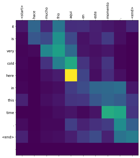
translate(u'hace mucho frio aqui en este momento.')
Input: <start> hace mucho frio aqui en este momento . <end>
Predicted translation: it is very cold here in this time . <end>
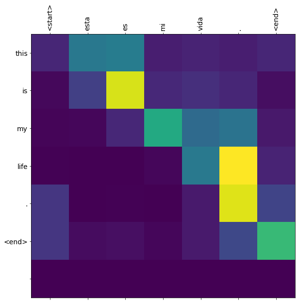
translate(u'esta es mi vida.')
Input: <start> esta es mi vida . <end>
Predicted translation: this is my life . <end>
Metrics in a real context#
From: wikipedia
BLEU (bilingual evaluation understudy) is an algorithm for evaluating the quality of text which has been machine-translated from one natural language to another. Quality is considered to be the correspondence between a machine’s output and that of a human: “the closer a machine translation is to a professional human translation, the better it is” – this is the central idea behind BLEU. BLEU was one of the first metrics to claim a high correlation with human judgements of quality, and remains one of the most popular automated and inexpensive metrics.
Scores are calculated for individual translated segments—generally sentences—by comparing them with a set of good quality reference translations. Those scores are then averaged over the whole corpus to reach an estimate of the translation’s overall quality. Intelligibility or grammatical correctness are not taken into account
NLTK provides the sentence_bleu() function for evaluating a candidate sentence against one or more reference sentences.