LAB 07.01 - Optimization for ML

!wget --no-cache -O init.py -q https://raw.githubusercontent.com/rramosp/ai4eng.v1/main/content/init.py
import init; init.init(force_download=False); init.get_weblink()

from local.lib.rlxmoocapi import submit, session
session.LoginSequence(endpoint=init.endpoint, course_id=init.course_id, lab_id="L07.01", varname="student");

from sklearn.datasets import make_moons
import numpy as np
import matplotlib.pyplot as plt
import pandas as pd
from local.lib import mlutils
%matplotlib inline

Dataset

you have data in a matrix \(\mathbf{X} \in \mathbb{R}^{m\times n}\) and the corresponding labels \(\mathbf{y} \in \mathbb{R}^m\).

each row in matrix \(\mathbf{X}\) contains one data point \(\mathbf{x}^{(i)}\)

\[\begin{split}\begin{bmatrix} x^{(0)}\\ x^{(1)}\\ ... \\ x^{(m-1)} \end{bmatrix} \end{split}\]

and each data point is a vector \(\mathbf{x}^{(i)}=[x^{(i)}_0, x^{(i)}_1,...,x^{(i)}_{n-1}]\).

Also, each data point has an associated label \(\mathbf{y} = [y^{(0)}, y^{(1)},..., y^{(m-1)}]\).

We will be doing binary classification so \(y^{(0)}\in \{0,1\}\)

d = pd.read_csv("local/data/moons.csv")
X = d[["col1", "col2"]].values
y = d["target"].values
print ("m=%d\nn=%d"%(X.shape[0], X.shape[1]))
X.shape, y.shape

m=200
n=2

((200, 2), (200,))

print (X[:10])
print (y[:10])

[[ 1.303374   -0.81478084]
 [-0.98727894 -0.06456482]
 [ 2.317555    0.44925394]
 [ 0.85310268 -0.22083508]
 [-0.97006406  0.64095693]
 [ 1.65849049 -0.2342485 ]
 [ 0.8684624  -0.28940167]
 [ 0.05631143  0.00296565]
 [ 0.88824669 -0.12888889]
 [ 0.9925954   0.31451716]]
[1 0 1 1 0 1 1 1 1 0]

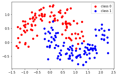
plt.scatter(X[:,0][y==0], X[:,1][y==0], color="red", label="class 0")
plt.scatter(X[:,0][y==1], X[:,1][y==1], color="blue", label="class 1")
plt.legend();

Task 1: Create a prediction function

complete the following prediction function which accepts:

• \(\mathbf{\theta} = [\theta_0, \theta_1,... \theta_{n-1}] \in \mathbb{R}^n\), a numpy vector.

• \(b \in \mathbb{R}\) , a float.

• \(\mathbf{X} \in \mathbb{R}^{m\times n}\), a numpy 2D array.

and returns

• \(\hat{\mathbf{y}} = [\hat{y}^{(0)}, \hat{y}^{(1)}, ..., \hat{y}^{(m-1)}] \in \mathbb{R}^m\) defined as follows

\[\hat{y}^{(i)} = \text{sigm}(\mathbf{\theta} \cdot \mathbf{x}^{(i)} + b) = \text{sigm}(\theta_0 x^{(i)}_0 + \theta_1 x^{(i)}_1 + b)\]

with

\[\text{sigm}(z) = \frac{1}{1+e^{-z}}\]

note that we can also express the prediction vector \(\hat{\mathbf{y}}\) over the whole dataset as

\[\hat{\mathbf{y}} = \text{sigm}(\mathbf{\theta} \cdot \mathbf{X} + b)\]

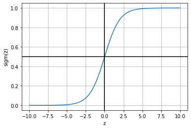
observe that for any \(z\), the sigmoid function squeshes its value between 0 and 1. It can be simply seen as a continuous step function which converts any negative value into 0, and any positive value into 1.

challenge: use only one line of python code (not counting the \(\text{sigm}\) definition)

warn: your function must work with any \(\mathbf{X} \in \mathbb{R}^{m\times n}\) and \(\mathbf{\theta} \in \mathbb{R}^n\), for any \(m\) and \(n\), not only for \(n=2\)

z = np.linspace(-10,10,100)
sigm = lambda x: 1/(1+np.exp(-x))
plt.plot(z, sigm(z)); plt.grid(); plt.xlabel("z"); plt.ylabel("sigm(z)")
plt.axhline(0.5, color="black"); plt.axvline(0, color="black")

<matplotlib.lines.Line2D at 0x7f23f42aedd0>

def prediction(t,b,X):
    sigm = lambda z: 1/(1+np.exp(-z))    
    yhat = .... # YOUR CODE HERE
    return yhat 

check manually your code. The following should yield a vector with 200 elements, whose sum should be 99.97 at its four first elements

[0.02328672 0.91257015 0.03781132 0.16139629 ... ]

t,b = np.r_[[-2,2]], 0.5
yhat = prediction(t,b,X)
print (yhat.shape)
print (np.sum(yhat))
print (yhat)

submit your code

student.submit_task(globals(), task_id="task_01");

Task 2: Create the loss function

accepting the following paramters

• \(\mathbf{\theta} = [\theta_0, \theta_1] \in \mathbb{R}^n\), a numpy vector.

• \(b \in \mathbb{R}\) , a float.

• \(\mathbf{X} \in \mathbb{R}^{m\times n}\), a numpy 2D array.

• \(\mathbf{y} \in \mathbb{R}^m\), a numpy vector.

\[\text{loss}(\theta, b, \mathbf{X} , \mathbf{y}) = \frac{1}{m}\sum_{i=0}^{m-1}(\hat{y}^{(i)}-y^{(i)})^2\]

challenge: use only one line of python (not counting the sigm and prediction functions).

def loss(t,b,X,y):
    sigm = lambda z: 1/(1+np.exp(-z))        
    result = ...
    return result

check manually your code, you should get a loss of 0.664 approx.

t,b = np.r_[[-2,2]], 0.5
loss(t,b,X,y)

submit your code

student.submit_task(globals(), task_id="task_02");

Task 3: Obtain the best \(\theta\) and \(b\) with black box optimization

Complete the following function so that it returns the best \(\theta\) and \(b\) for a given data set.

Observe that

• x0 in scipy.optimize.minimize must be a vector of three items, the first two corresponding to \(\theta_0\) and \(\theta_1\), and the last one to \(b\).

• the return value of the optimizer r.x will also contain three items, and you will have to separate the first two into t and the last one into b.

• you will have to adapt your loss function created before so that it extracts \(\theta\) and \(b\) from the variable params.

def fit(X,y):
    from scipy.optimize import minimize
    
    def loss(params):
        t = ... # extract t from params
        b = ... # extract b params
        sigm = lambda z: 1/(1+np.exp(-z))        
        return ... # your code here
    
    tinit = np.zeros(shape=X.shape[1]+1) # keep this initialization
    r = minimize(...) # complete the call to minimize
    t = ... # extract t from r.x
    b = ... # extract b from r.x
    return t, b

t, b = fit(X,y)

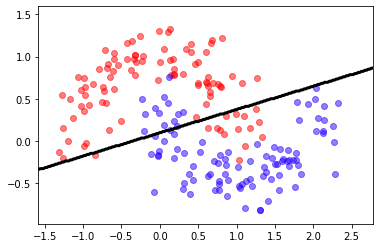
check manually your code, you should get an accuracy of about 84%-87%, and a classification frontier similar to this one.

Observe how we convert the sigmoid output which can be any number \(\in [0,1]\), into a discrete classification (0 or 1) by thresholding on 0.5

from IPython.display import Image
Image(filename='local/imgs/logregmoons.png')

t, b

mlutils.plot_2Ddata_with_boundary(lambda X: prediction(t,b,X)>.5, X, y)

acc = np.mean( (prediction(t,b,X)>.5)==y)
print ("accuracy %.3f"%acc)

submit your code

student.submit_task(globals(), task_id="task_03");