04.02 - DATA CLEANING

!wget --no-cache -O init.py -q https://raw.githubusercontent.com/rramosp/ai4eng.v1/main/content/init.py
import init; init.init(force_download=False); init.get_weblink()

Based on Kaggle House Pricing Prediction Competition

• Inspect and learn from the competition Notebooks

• You must make available to this notebook the train.csv file from the competition data section. If running this notebook in Google Colab you must upload it in the notebook files section in Colab.

## KEEPOUTPUT
import pandas as pd
import seaborn as sns
import numpy as np
import matplotlib.pyplot as plt
from progressbar import progressbar as pbar
from local.lib import mlutils
%matplotlib inline
d = pd.read_csv("train.csv", index_col="Id")
d.head()

	MSSubClass	MSZoning	LotFrontage	LotArea	Street	Alley	LotShape	LandContour	Utilities	LotConfig	...	PoolArea	PoolQC	Fence	MiscFeature	MiscVal	MoSold	YrSold	SaleType	SaleCondition	SalePrice
Id
1	60	RL	65.0	8450	Pave	NaN	Reg	Lvl	AllPub	Inside	...	0	NaN	NaN	NaN	0	2	2008	WD	Normal	208500
2	20	RL	80.0	9600	Pave	NaN	Reg	Lvl	AllPub	FR2	...	0	NaN	NaN	NaN	0	5	2007	WD	Normal	181500
3	60	RL	68.0	11250	Pave	NaN	IR1	Lvl	AllPub	Inside	...	0	NaN	NaN	NaN	0	9	2008	WD	Normal	223500
4	70	RL	60.0	9550	Pave	NaN	IR1	Lvl	AllPub	Corner	...	0	NaN	NaN	NaN	0	2	2006	WD	Abnorml	140000
5	60	RL	84.0	14260	Pave	NaN	IR1	Lvl	AllPub	FR2	...	0	NaN	NaN	NaN	0	12	2008	WD	Normal	250000

5 rows × 80 columns

## KEEPOUTPUT
print (d.shape)

(1460, 80)

We must repair the missing data in the following columns

Possible repair actions:

• Remove row or column

• Replace value (why what?)

## KEEPOUTPUT
k = d.isna().sum()
k[k!=0]

LotFrontage      259
Alley           1369
MasVnrType       872
MasVnrArea         8
BsmtQual          37
BsmtCond          37
BsmtExposure      38
BsmtFinType1      37
BsmtFinType2      38
Electrical         1
FireplaceQu      690
GarageType        81
GarageYrBlt       81
GarageFinish      81
GarageQual        81
GarageCond        81
PoolQC          1453
Fence           1179
MiscFeature     1406
dtype: int64

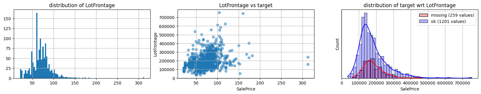
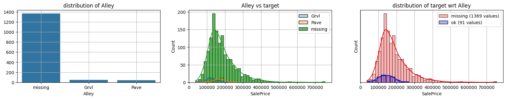
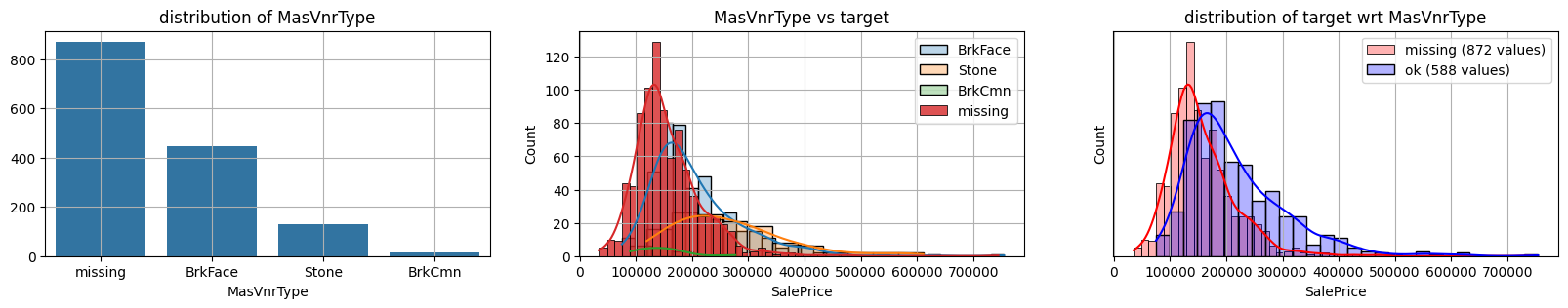
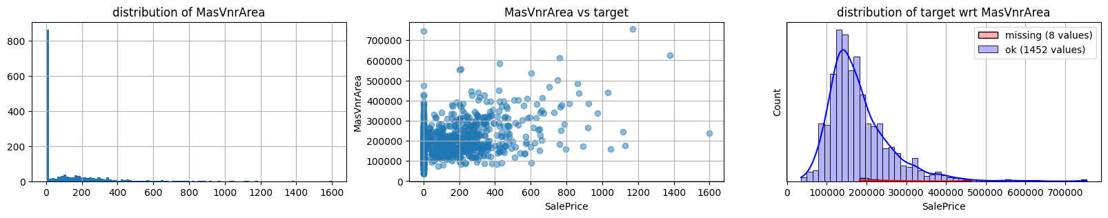
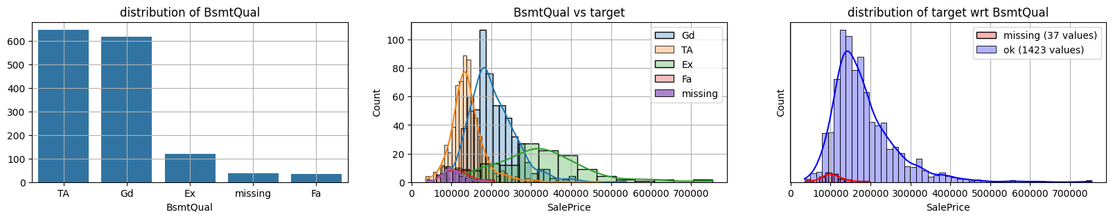
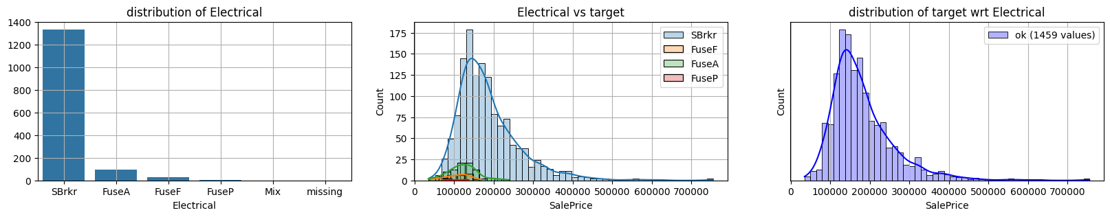
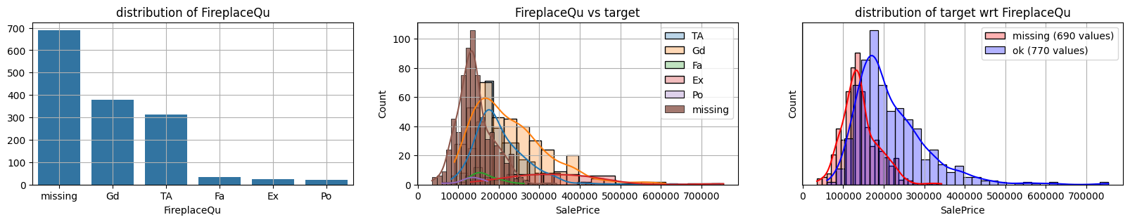
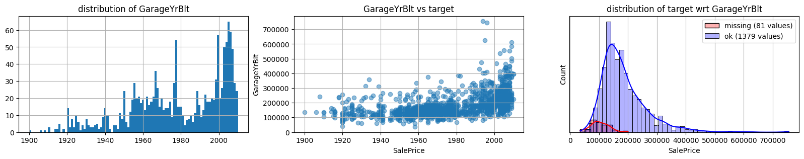
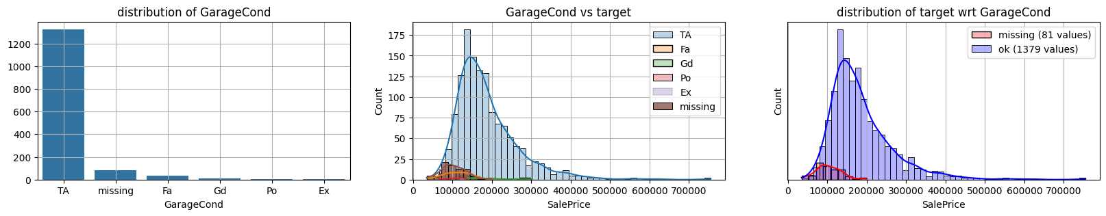
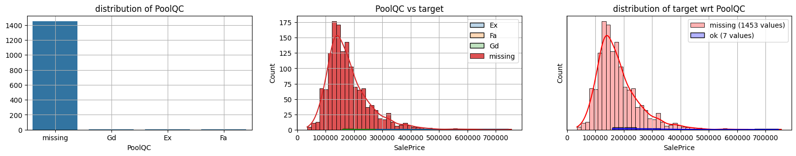
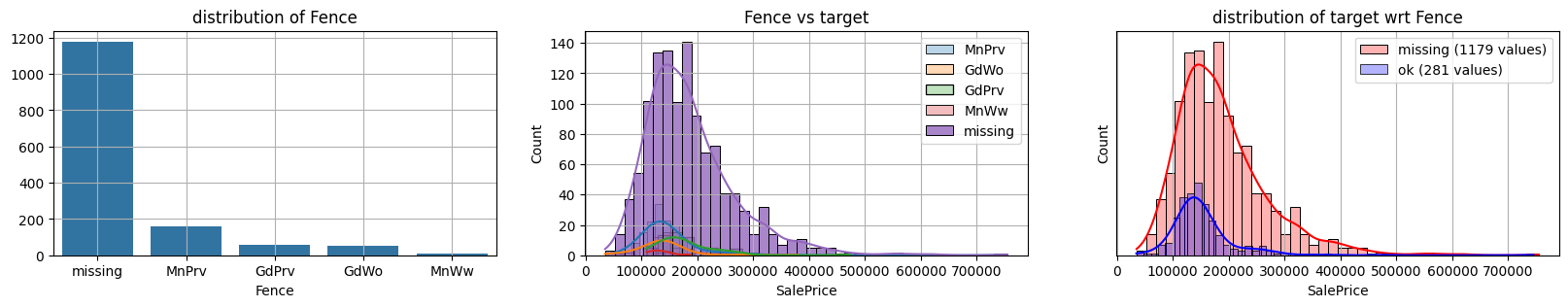
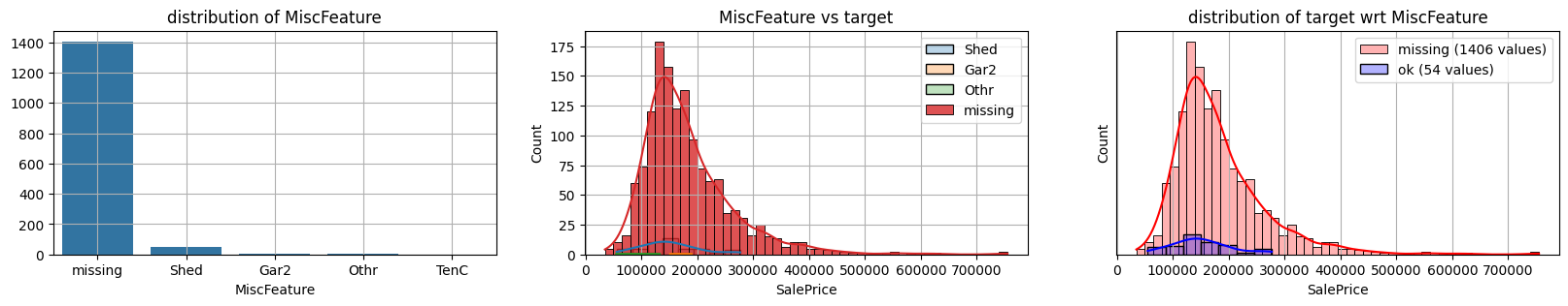
Inspect and understand missing data

## KEEPOUTPUT
def plot_missing(col, target):

    def f1():

        if d[col].dtype==object:
            k = d[col].fillna("missing").value_counts()
            sns.barplot(x=k.index, y=k.values)
        else:
            plt.hist(d[col].dropna().values, bins=100)
        plt.title("distribution of %s"%col)
        plt.grid()

    def f2():
        if d[col].dtype==object:
            k=d[[col,target]].dropna()
            for v in d[col].dropna().unique():
                if sum(k[col]==v)>1:
                    sns.histplot(k[target][k[col]==v], kde=True,
                                 label=v, alpha=.3);
            if sum(d[col].isna())>1:
                sns.histplot(d[target][d[col].isna()],
                             alpha=.8, kde=True,
                             label="missing")
            plt.legend();
        else:
            plt.scatter(d[col], d[target], alpha=.5)
            plt.xlabel(target)
            plt.ylabel(col)
        plt.grid()
        plt.title("%s vs target"%(col))

    def f3():
        n = np.sum(d[col].isna())
        if n>1:
            sns.histplot(d[target][d[col].isna()], color="red", kde=True, alpha=.3, label="missing (%d values)"%n)
        sns.histplot(d[target][~d[col].isna()], color="blue", kde=True, alpha=.3, label="ok (%d values)"%(len(d)-n))
        plt.title("distribution of target wrt %s"%col)
        plt.yticks([])
        plt.grid()
        plt.legend()

    mlutils.figures_grid(3,1, [f1, f2, f3], figsize=(20,3))

## KEEPOUTPUT
for col in k[k!=0].index:
    plot_missing(col, target="SalePrice")

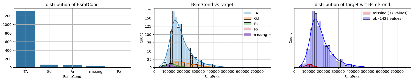
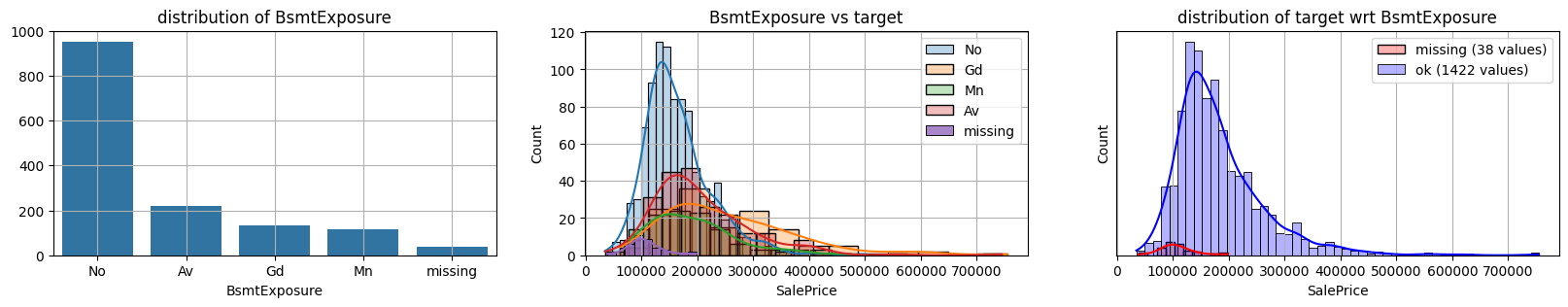
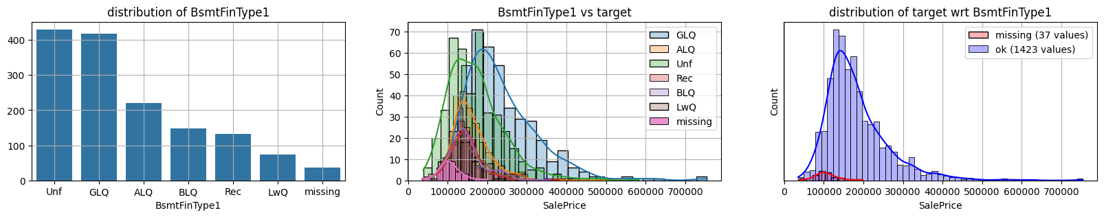
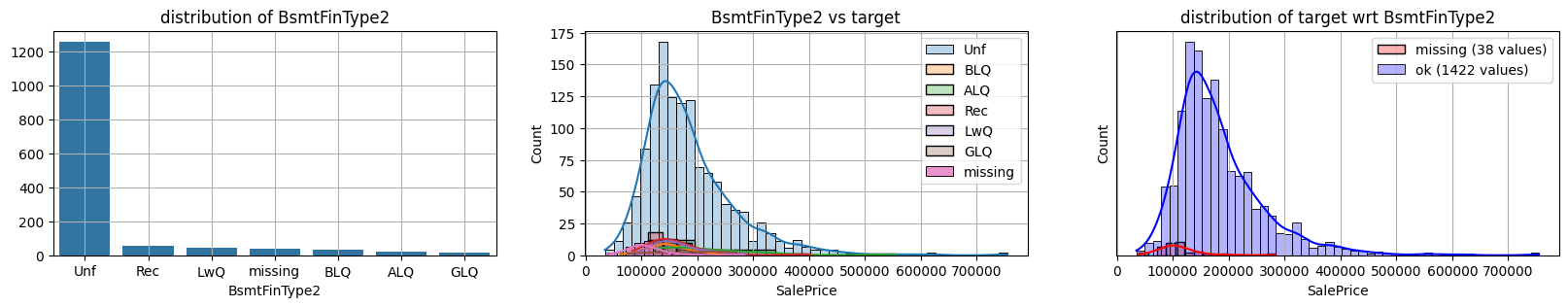
common sense

• too many missing data in Alley. Information might only help non-missing items with little impact on

• missing data in Bsmt* seem all the same

• missing data in Garage* sell all the same

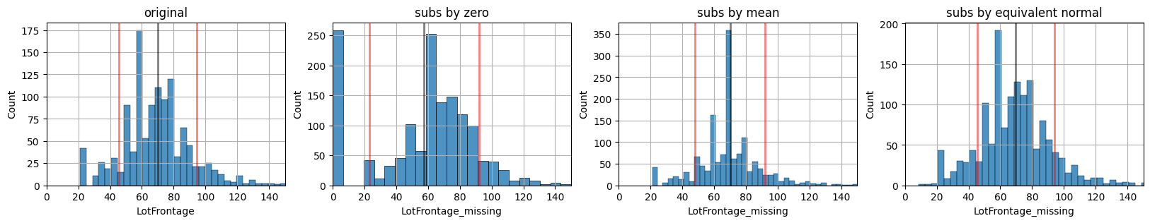
For continuous variables

Three substitution techniques

• by a fixed value (zero)

• by a fixed value (the mean)

• sampling from an equivalent normal (same mean and std)

First we create the different datasets:

• dn: original data only with numerical attributes

• dl0: substituting missing values with zero

• dlm: substituting missing values with the mean

• dlr: substituting missing values with an equivalent normal (same mean and stdev)

def xdistplot(k, title="", xlim=None):
    vals = k
    sns.histplot(k, alpha= .8);
    m,s = np.mean(vals), np.std(vals)
    plt.axvline(m, color="black", lw=2, alpha=.5)
    plt.axvline(m+s, color="red", lw=2, alpha=.5)
    plt.axvline(m-s, color="red", lw=2, alpha=.5)
    x = np.linspace(np.min(vals), np.max(vals), 100)
    plt.title(title)
    plt.grid();
    if xlim is not None:
        plt.xlim(xlim)

def subs_policies(d, col):
    mcol = "%s_missing"%col
    dn = d.T.dropna().T
    dn = dn[[i for i in dn.columns if d[i].dtype!=object]]
    print (dn.shape)

    na_idxs = np.argwhere(d[col].isna().values)[:,0]

    dl0 = dn.copy()
    dlm = dn.copy()
    dlr = dn.copy()

    dl0[mcol] = d[col].fillna(0)
    dlm[mcol] = d[col].fillna( d[col].mean())

    k = d[col].copy()
    k[k.isna()] = np.random.normal(loc=np.mean(k), scale=np.std(k), size=np.sum(k.isna()))
    dlr[mcol] = k

    f0 = lambda: xdistplot(d[col].dropna(), "original", [0,150])
    f1 = lambda: xdistplot(dl0[mcol], "subs by zero", [0,150])
    f2 = lambda: xdistplot(dlm[mcol], "subs by mean", [0,150])
    f3 = lambda: xdistplot(dlr[mcol], "subs by equivalent normal", [0,150])

    mlutils.figures_grid(4,1, [f0, f1, f2, f3], figsize=(20,3))
    return dn, dl0, dlm, dlr, na_idxs

## KEEPOUTPUT
dn, dl0, dlm, dlr, na_idxs = subs_policies(d, "LotFrontage")

(1460, 34)

Validation workflow for repairing missing values on LotFrontage

Which policy for repairing missing data is best?

Short answer: we do not know \(\rightarrow\) we must seek evidence

We will now integrate them in an ML workflow, creating predictive models and seeking for evidence if models improve or not when using different policies for repairing missing data.

We train a lot of models (resampling training data) with each dataset and then run a classical hypothesis test on model performance:

• \(e_1\): control group, models trained without LotFrontage

• \(e_2\): population group, models trained with LotFrontage with fillna=0

Our null hypothesis (there is no effect in using the new variable):

\[H_0: \mu_{e_1}-\mu_{e_2}=0 \Rightarrow \mu_{e_1-e_2}=0\]

Our test hypothesis (including fillna=0 improves models):

\[H_1: \mu_{e_1}-\mu_{e_2}<0 \Rightarrow \mu_{e_1-e_2}<0\]

from sklearn.model_selection import cross_val_score, ShuffleSplit
from sklearn.ensemble import RandomForestRegressor
from sklearn.metrics import mean_absolute_error, make_scorer
from scipy.stats import ttest_ind

def getXY (dn):
    xcols = [i for i in dn.columns if i!="SalePrice"]
    X = dn[xcols].values.astype(float)
    y = dn.SalePrice.values.astype(float)
    return X,y,xcols

def experiment(dn, estimator, n_models=20, test_size=.3):
    X,y,_ = getXY(dn)
    r = cross_val_score(estimator, X, y, cv=ShuffleSplit(n_models, test_size=test_size),
                        scoring=make_scorer(mean_absolute_error))
    return r

def HTest(ref_dataset, h_datasets, n_models=30, experiment=experiment, **kwargs):
    estimator = RandomForestRegressor(n_estimators=20)
    re = [experiment(i, estimator, n_models=n_models, **kwargs) for i in pbar([ref_dataset]+h_datasets)]

    for r in re[1:]:
        print (ttest_ind(re[0],r))

## KEEPOUTPUT
dl0.head()

	MSSubClass	LotArea	OverallQual	OverallCond	YearBuilt	YearRemodAdd	BsmtFinSF1	BsmtFinSF2	BsmtUnfSF	TotalBsmtSF	...	OpenPorchSF	EnclosedPorch	3SsnPorch	ScreenPorch	PoolArea	MiscVal	MoSold	YrSold	SalePrice	LotFrontage_missing
Id
1	60	8450	7	5	2003	2003	706	0	150	856	...	61	0	0	0	0	0	2	2008	208500	65.0
2	20	9600	6	8	1976	1976	978	0	284	1262	...	0	0	0	0	0	0	5	2007	181500	80.0
3	60	11250	7	5	2001	2002	486	0	434	920	...	42	0	0	0	0	0	9	2008	223500	68.0
4	70	9550	7	5	1915	1970	216	0	540	756	...	35	272	0	0	0	0	2	2006	140000	60.0
5	60	14260	8	5	2000	2000	655	0	490	1145	...	84	0	0	0	0	0	12	2008	250000	84.0

5 rows × 35 columns

## KEEPOUTPUT
HTest(dn, [dl0, dlm, dlr], n_models=50)

100% (4 of 4) |##########################| Elapsed Time: 0:00:49 Time:  0:00:49

TtestResult(statistic=-1.3541252006646298, pvalue=0.1788107411367549, df=98.0)
TtestResult(statistic=-0.6937964889158504, pvalue=0.48945111677260755, df=98.0)
TtestResult(statistic=-0.5677251272549229, pvalue=0.5715199997392869, df=98.0)

## KEEPOUTPUT
HTest(dn, [dl0, dlm, dlr], n_models=50)

100% (4 of 4) |##########################| Elapsed Time: 0:00:49 Time:  0:00:49

TtestResult(statistic=-0.37511561454083137, pvalue=0.7083850959273256, df=98.0)
TtestResult(statistic=-0.3321948468400306, pvalue=0.7404516048445651, df=98.0)
TtestResult(statistic=0.4780530200131818, pvalue=0.6336771343561804, df=98.0)

No \(p\) value is really significative so the different substitution policies do no help improve overall in this simplified setting. More over, repeated experiments show to evidence of any approach better than others (always better \(p\) value)

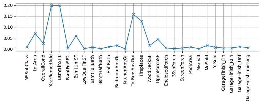
Some models provide us with a measure of feature importance. Observe the behaviour of the most important variables in the scatter matrix plot of previous notebook.

## KEEPOUTPUT
X, y, xcols = getXY(dlr)
rf = RandomForestRegressor(n_estimators=20)
rf.fit(X,y);
plt.figure(figsize=(10,2)); plt.grid()
plt.plot(rf.feature_importances_, label="est1", marker="x")
plt.xticks(range(len(xcols)), xcols, rotation="vertical");

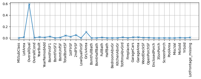
so somehow it is understandable that providing values for this missing variable does not have so much impact.

We could try to see ONLY how records with THIS missing data behave. Observe that na_idxs marks which rows contain na values so that they are used to measure validation performance.

There is still no clear evidence that any filling strategy for missing values is better than other.

def na_cross_val_score(estimator, X, y, cv, scoring, val_idxs):
    r = []
    for tr_idxs, ts_idxs in cv.split(X):
        tr_idxs, ts_idxs = np.r_[tr_idxs], np.r_[ts_idxs]
        rf.fit(X[tr_idxs], y[tr_idxs])
        valts_idxs = np.r_[[i for i in ts_idxs if i in val_idxs]]
        r.append(scoring(rf, X[valts_idxs], y[valts_idxs]))
    return r


def na_experiment(dn, estimator, na_idxs, n_models=20, test_size=.3):
    X,y,_ = getXY(dn)
    r = na_cross_val_score(estimator, X, y, cv=ShuffleSplit(n_models, test_size=test_size),
                        scoring=make_scorer(mean_absolute_error), val_idxs=na_idxs)
    return r

## KEEPOUTPUT
HTest(dn, [dl0, dlm, dlr], experiment=na_experiment, na_idxs=na_idxs, n_models=50)

100% (4 of 4) |##########################| Elapsed Time: 0:00:49 Time:  0:00:49

TtestResult(statistic=-2.5660466465640033, pvalue=0.011800717881861248, df=98.0)
TtestResult(statistic=-2.053620290722926, pvalue=0.042675908653560114, df=98.0)
TtestResult(statistic=-1.5568314871351756, pvalue=0.12273414960890429, df=98.0)

HTest(dn, [dl0, dlm, dlr], experiment=na_experiment, na_idxs=na_idxs, n_models=50)

100% (4 of 4) |##########################| Elapsed Time: 0:00:49 Time:  0:00:49

TtestResult(statistic=-1.4547828358181458, pvalue=0.14892498057497006, df=98.0)
TtestResult(statistic=-0.5523471899998421, pvalue=0.5819680699474099, df=98.0)
TtestResult(statistic=-1.4511464404586971, pvalue=0.14993266003326222, df=98.0)

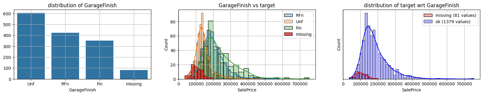
For categorical features

• we must convert them to numerical

  • if categories are ordered \(\rightarrow\) convert to positive integer

  • otherwise \(\rightarrow\) convert to one hot

• we must decide on missing values:

  • remove row or column

  • assign an existing value

  • assign a new value

## KEEPOUTPUT
col = "GarageFinish"
print ("missing", sum(d[col].isna()))
d[col].value_counts()

missing 81

GarageFinish
Unf    605
RFn    422
Fin    352
Name: count, dtype: int64

def to_onehot(x):
    values = np.unique(x)
    r = np.r_[[np.argwhere(i==values)[0][0] for i in x]]
    return np.eye(len(values))[r].astype(int)

def replace_column_with_onehot(d, col):
    assert sum(d[col].isna())==0, "column must have no NaN values"
    values = np.unique(d[col]
                      )
    k = to_onehot(d[col].values)
    r = pd.DataFrame(k, columns=["%s_%s"%(col, values[i]) for i in range(k.shape[1])], index=d.index).join(d)
    del(r[col])
    return r

observe onehot encoding

## KEEPOUTPUT
d[[col]].head(10)

	GarageFinish
Id
1	RFn
2	RFn
3	RFn
4	Unf
5	RFn
6	Unf
7	RFn
8	RFn
9	Unf
10	RFn

## KEEPOUTPUT
replace_column_with_onehot(d[[col]].dropna().copy(), col).head(10)

	GarageFinish_Fin	GarageFinish_RFn	GarageFinish_Unf
Id
1	0	1	0
2	0	1	0
3	0	1	0
4	0	0	1
5	0	1	0
6	0	0	1
7	0	1	0
8	0	1	0
9	0	0	1
10	0	1	0

we now create a onehot encoding for each case:

• create a separate value for missing data

• set missing data to an existing category. In this case we will set it to the closest category distribution wrt the target variable according the plots above

## KEEPOUTPUT
rm1 = replace_column_with_onehot(d[[col]].fillna("missing").copy(), col)
rm2 = replace_column_with_onehot(d[[col]].fillna("Unf").copy(), col)

## KEEPOUTPUT
rm1.head()

	GarageFinish_Fin	GarageFinish_RFn	GarageFinish_Unf	GarageFinish_missing
Id
1	0	1	0	0
2	0	1	0	0
3	0	1	0	0
4	0	0	1	0
5	0	1	0	0

## KEEPOUTPUT
rm2.head()

	GarageFinish_Fin	GarageFinish_RFn	GarageFinish_Unf
Id
1	0	1	0
2	0	1	0
3	0	1	0
4	0	0	1
5	0	1	0

## KEEPOUTPUT
dm1 = dn.join(rm1)
dm2 = dn.join(rm2)
dm1.shape, dm2.shape

((1460, 38), (1460, 37))

again, do hypothesis testing to seek for evidence for improvements for any of the methods

## KEEPOUTPUT
HTest(dn, [dm1, dm2], experiment=experiment, n_models=50)

100% (3 of 3) |##########################| Elapsed Time: 0:00:38 Time:  0:00:38

TtestResult(statistic=-0.7343576845947623, pvalue=0.4644842464733756, df=98.0)
TtestResult(statistic=-0.35926068145867207, pvalue=0.7201730079370724, df=98.0)

## KEEPOUTPUT
na_idxs = np.argwhere(d[col].isna().values)[:,0]
HTest(dn, [dm1, dm2], experiment=na_experiment, na_idxs=na_idxs, n_models=50)

100% (3 of 3) |##########################| Elapsed Time: 0:00:37 Time:  0:00:37

TtestResult(statistic=2.0301224227097934, pvalue=0.045054029061182464, df=98.0)
TtestResult(statistic=1.1337018450245944, pvalue=0.25968538695450255, df=98.0)

Again, no \(p\) value is sufficiently significative to provide evidence for improved classification alone. However, approach number 2 (substituting missing data with Unf) does seem to consistently get better \(p\) value and, thus, more chance to improve performance when combined with other data cleaning choices.

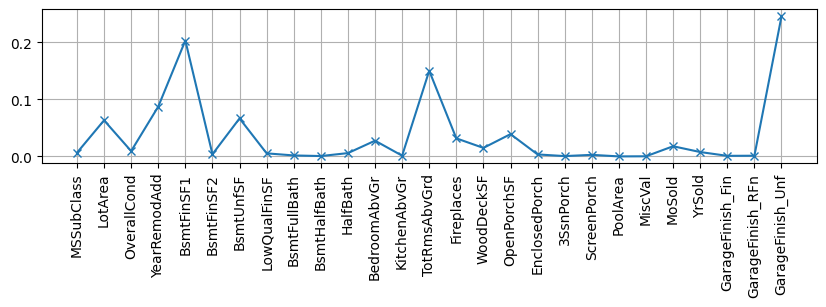
Observe also how the missing category dilutes the importance of Unf after other variables are taken out.

## KEEPOUTPUT
dk = dm2.copy()
dk = dk[[i for i in dm2.columns if not i in ["OverallQual", "GarageCars", "GrLivArea",
                                             "GarageArea", "YearBuilt", "TotalBsmtSF",
                                            "1stFlrSF", "2ndFlrSF", "FullBath"]]]
X, y, xcols = getXY(dk)
rf = RandomForestRegressor(n_estimators=10)
rf.fit(X,y);
plt.figure(figsize=(10,2)); plt.grid()
plt.plot(rf.feature_importances_, label="est1", marker="x")
plt.xticks(range(len(xcols)), xcols, rotation="vertical");

## KEEPOUTPUT
dk = dm1.copy()
dk = dk[[i for i in dm1.columns if not i in ["OverallQual", "GarageCars", "GrLivArea",
                                             "GarageArea", "YearBuilt", "TotalBsmtSF",
                                            "1stFlrSF", "2ndFlrSF", "FullBath"]]]
X, y, xcols = getXY(dk)
rf = RandomForestRegressor(n_estimators=10)
rf.fit(X,y);
plt.figure(figsize=(10,2)); plt.grid()
plt.plot(rf.feature_importances_, label="est1", marker="x")
plt.xticks(range(len(xcols)), xcols, rotation="vertical");