02.04 - PANDAS

!wget --no-cache -O init.py -q https://raw.githubusercontent.com/rramosp/ai4eng.v1/main/content/init.py
import init; init.init(force_download=False); init.get_weblink()

import numpy as np
import pandas as pd
import matplotlib.pyplot as plt
%matplotlib inline

pandas is mostly about manipulating tables of data

see this cheat sheet: https://pandas.pydata.org/Pandas_Cheat_Sheet.pdf

Pandas main object is a DataFrame

• can read .csv, .excel, etc.

!head local/data/internet_facebook.dat

# Pais,Uso_Internet,Uso_Facebook
Argentina,49.40,30.53
Australia,80.60,46.01
Belgium,67.30,36.98
Brazil,37.76,4.39
Canada,72.30,52.08
Chile,50.90,46.14
China,22.40,0.05
Colombia,38.80,25.90
Egypt,12.90,5.68

!wc local/data/weather_data_austin_2010.csv

  8760  17519 254046 local/data/weather_data_austin_2010.csv

df = pd.read_csv('local/data/internet_facebook.dat', index_col='# Pais')
df

	Uso_Internet	Uso_Facebook
# Pais
Argentina	49.40	30.53
Australia	80.60	46.01
Belgium	67.30	36.98
Brazil	37.76	4.39
Canada	72.30	52.08
Chile	50.90	46.14
China	22.40	0.05
Colombia	38.80	25.90
Egypt	12.90	5.68
France	65.70	32.91
Germany	67.00	14.07
Hong_Kong	69.50	52.33
India	7.10	1.52
Indonesia	10.50	13.49
Italy	48.80	30.62
Japan	73.80	2.00
Malaysia	62.80	37.77
Mexico	24.90	16.80
Netherlands	82.90	20.54
Peru	26.20	13.34
Philippines	21.50	19.68
Poland	52.00	11.79
Russia	27.00	2.99
Saudi_Arabia	22.70	11.65
South_Africa	10.50	7.83
Spain	66.80	30.24
Sweden	80.70	44.72
Taiwan	66.10	38.21
Thailand	20.50	10.29
Turkey	35.00	31.91
USA	77.33	46.98
UK	70.18	45.97
Venezuela	25.50	28.64

df.head()

	Uso_Internet	Uso_Facebook
# Pais
Argentina	49.40	30.53
Australia	80.60	46.01
Belgium	67.30	36.98
Brazil	37.76	4.39
Canada	72.30	52.08

df.tail()

	Uso_Internet	Uso_Facebook
# Pais
Thailand	20.50	10.29
Turkey	35.00	31.91
USA	77.33	46.98
UK	70.18	45.97
Venezuela	25.50	28.64

df.columns

Index(['Uso_Internet', 'Uso_Facebook'], dtype='object')

df.index

Index(['Argentina', 'Australia', 'Belgium', 'Brazil', 'Canada', 'Chile',
       'China', 'Colombia', 'Egypt', 'France', 'Germany', 'Hong_Kong', 'India',
       'Indonesia', 'Italy', 'Japan', 'Malaysia', 'Mexico', 'Netherlands',
       'Peru', 'Philippines', 'Poland', 'Russia', 'Saudi_Arabia',
       'South_Africa', 'Spain', 'Sweden', 'Taiwan', 'Thailand', 'Turkey',
       'USA', 'UK', 'Venezuela'],
      dtype='object', name='# Pais')

fix the index name

df.index.name="Pais"
df.head()

	Uso_Internet	Uso_Facebook
Pais
Argentina	49.40	30.53
Australia	80.60	46.01
Belgium	67.30	36.98
Brazil	37.76	4.39
Canada	72.30	52.08

df.describe()

	Uso_Internet	Uso_Facebook
count	33.000000	33.000000
mean	46.890000	24.668182
std	24.456421	16.511662
min	7.100000	0.050000
25%	24.900000	11.650000
50%	49.400000	25.900000
75%	67.300000	37.770000
max	82.900000	52.330000

df.info()

<class 'pandas.core.frame.DataFrame'>
Index: 33 entries, Argentina to Venezuela
Data columns (total 2 columns):
Uso_Internet    33 non-null float64
Uso_Facebook    33 non-null float64
dtypes: float64(2)
memory usage: 792.0+ bytes

a dataframe is made of Series. Observe that each series has its own type

s1 = df["Uso_Internet"]
type(s1)

pandas.core.series.Series

s1

Pais
Argentina       49.40
Australia       80.60
Belgium         67.30
Brazil          37.76
Canada          72.30
Chile           50.90
China           22.40
Colombia        38.80
Egypt           12.90
France          65.70
Germany         67.00
Hong_Kong       69.50
India            7.10
Indonesia       10.50
Italy           48.80
Japan           73.80
Malaysia        62.80
Mexico          24.90
Netherlands     82.90
Peru            26.20
Philippines     21.50
Poland          52.00
Russia          27.00
Saudi_Arabia    22.70
South_Africa    10.50
Spain           66.80
Sweden          80.70
Taiwan          66.10
Thailand        20.50
Turkey          35.00
USA             77.33
UK              70.18
Venezuela       25.50
Name: Uso_Internet, dtype: float64

if the column name is not too fancy (empy spaces, accents, etc.) we can use columns names as python syntax.

df.Uso_Facebook

Pais
Argentina       30.53
Australia       46.01
Belgium         36.98
Brazil           4.39
Canada          52.08
Chile           46.14
China            0.05
Colombia        25.90
Egypt            5.68
France          32.91
Germany         14.07
Hong_Kong       52.33
India            1.52
Indonesia       13.49
Italy           30.62
Japan            2.00
Malaysia        37.77
Mexico          16.80
Netherlands     20.54
Peru            13.34
Philippines     19.68
Poland          11.79
Russia           2.99
Saudi_Arabia    11.65
South_Africa     7.83
Spain           30.24
Sweden          44.72
Taiwan          38.21
Thailand        10.29
Turkey          31.91
USA             46.98
UK              45.97
Venezuela       28.64
Name: Uso_Facebook, dtype: float64

DataFrame indexing

is NOT exactly like numpy

• first index

  • if string refers to columns

  • if Series of booleans is used as a filter

• for selecting columns:

  • use .loc to select by Index

  • use .iloc to select by position

df["Colombia"]

---------------------------------------------------------------------
KeyError                            Traceback (most recent call last)
/opt/anaconda3/envs/p37/lib/python3.7/site-packages/pandas/core/indexes/base.py in get_loc(self, key, method, tolerance)
   2896             try:
-> 2897                 return self._engine.get_loc(key)
   2898             except KeyError:

pandas/_libs/index.pyx in pandas._libs.index.IndexEngine.get_loc()

pandas/_libs/index.pyx in pandas._libs.index.IndexEngine.get_loc()

pandas/_libs/hashtable_class_helper.pxi in pandas._libs.hashtable.PyObjectHashTable.get_item()

pandas/_libs/hashtable_class_helper.pxi in pandas._libs.hashtable.PyObjectHashTable.get_item()

KeyError: 'Colombia'

During handling of the above exception, another exception occurred:

KeyError                            Traceback (most recent call last)
<ipython-input-251-5f701fabe22b> in <module>
----> 1 df["Colombia"]

/opt/anaconda3/envs/p37/lib/python3.7/site-packages/pandas/core/frame.py in __getitem__(self, key)
   2993             if self.columns.nlevels > 1:
   2994                 return self._getitem_multilevel(key)
-> 2995             indexer = self.columns.get_loc(key)
   2996             if is_integer(indexer):
   2997                 indexer = [indexer]

/opt/anaconda3/envs/p37/lib/python3.7/site-packages/pandas/core/indexes/base.py in get_loc(self, key, method, tolerance)
   2897                 return self._engine.get_loc(key)
   2898             except KeyError:
-> 2899                 return self._engine.get_loc(self._maybe_cast_indexer(key))
   2900         indexer = self.get_indexer([key], method=method, tolerance=tolerance)
   2901         if indexer.ndim > 1 or indexer.size > 1:

pandas/_libs/index.pyx in pandas._libs.index.IndexEngine.get_loc()

pandas/_libs/index.pyx in pandas._libs.index.IndexEngine.get_loc()

pandas/_libs/hashtable_class_helper.pxi in pandas._libs.hashtable.PyObjectHashTable.get_item()

pandas/_libs/hashtable_class_helper.pxi in pandas._libs.hashtable.PyObjectHashTable.get_item()

KeyError: 'Colombia'

df.loc["Colombia"]

Uso_Internet    38.8
Uso_Facebook    25.9
Name: Colombia, dtype: float64

Index semantics is exact!!

df.loc["Colombia":"Spain"]

	Uso_Internet	Uso_Facebook
Pais
Colombia	38.8	25.90
Egypt	12.9	5.68
France	65.7	32.91
Germany	67.0	14.07
Hong_Kong	69.5	52.33
India	7.1	1.52
Indonesia	10.5	13.49
Italy	48.8	30.62
Japan	73.8	2.00
Malaysia	62.8	37.77
Mexico	24.9	16.80
Netherlands	82.9	20.54
Peru	26.2	13.34
Philippines	21.5	19.68
Poland	52.0	11.79
Russia	27.0	2.99
Saudi_Arabia	22.7	11.65
South_Africa	10.5	7.83
Spain	66.8	30.24

df.iloc[10:15]

	Uso_Internet	Uso_Facebook
Pais
Germany	67.0	14.07
Hong_Kong	69.5	52.33
India	7.1	1.52
Indonesia	10.5	13.49
Italy	48.8	30.62

filtering

df[df.Uso_Internet>80]

	Uso_Internet	Uso_Facebook
Pais
Australia	80.6	46.01
Netherlands	82.9	20.54
Sweden	80.7	44.72

combined conditions

df[(df.Uso_Internet>50)&(df.Uso_Facebook>50)]

	Uso_Internet	Uso_Facebook
Pais
Canada	72.3	52.08
Hong_Kong	69.5	52.33

df[(df.Uso_Internet>50)|(df.Uso_Facebook>50)]

	Uso_Internet	Uso_Facebook
Pais
Australia	80.60	46.01
Belgium	67.30	36.98
Canada	72.30	52.08
Chile	50.90	46.14
France	65.70	32.91
Germany	67.00	14.07
Hong_Kong	69.50	52.33
Japan	73.80	2.00
Malaysia	62.80	37.77
Netherlands	82.90	20.54
Poland	52.00	11.79
Spain	66.80	30.24
Sweden	80.70	44.72
Taiwan	66.10	38.21
USA	77.33	46.98
UK	70.18	45.97

Managing data

observe csv structure:

• missing column name

• missing data

!head local/data/comptagevelo2009.csv

Date,,Berri1,Maisonneuve_1,Maisonneuve_2,Brébeuf
01/01/2009,00:00,29,20,35,
02/01/2009,00:00,19,3,22,
03/01/2009,00:00,24,12,22,
04/01/2009,00:00,24,8,15,
05/01/2009,00:00,120,111,141,
06/01/2009,00:00,261,146,236,
07/01/2009,00:00,60,33,80,
08/01/2009,00:00,24,14,14,
09/01/2009,00:00,35,20,32,

d = pd.read_csv("local/data/comptagevelo2009.csv")
d

	Date	Unnamed: 1	Berri1	Maisonneuve_1	Maisonneuve_2	Brébeuf
0	01/01/2009	00:00	29	20	35	NaN
1	02/01/2009	00:00	19	3	22	NaN
2	03/01/2009	00:00	24	12	22	NaN
3	04/01/2009	00:00	24	8	15	NaN
4	05/01/2009	00:00	120	111	141	NaN
...	...	...	...	...	...	...
360	27/12/2009	00:00	66	29	52	0.0
361	28/12/2009	00:00	61	41	99	0.0
362	29/12/2009	00:00	89	52	115	0.0
363	30/12/2009	00:00	76	43	115	0.0
364	31/12/2009	00:00	53	46	112	0.0

365 rows × 6 columns

d.columns, d.shape

(Index(['Date', 'Unnamed: 1', 'Berri1', 'Maisonneuve_1', 'Maisonneuve_2',
        'Brébeuf'],
       dtype='object'), (365, 6))

numerical features

d.describe()

	Berri1	Maisonneuve_1	Maisonneuve_2	Brébeuf
count	365.000000	365.000000	365.000000	178.000000
mean	2032.200000	1060.252055	2093.169863	2576.359551
std	1878.879799	1079.533086	1854.368523	2484.004743
min	0.000000	0.000000	0.000000	0.000000
25%	194.000000	90.000000	228.000000	0.000000
50%	1726.000000	678.000000	1686.000000	1443.500000
75%	3540.000000	1882.000000	3520.000000	4638.000000
max	6626.000000	4242.000000	6587.000000	7575.000000

d["Berri1"].head()

0     29
1     19
2     24
3     24
4    120
Name: Berri1, dtype: int64

d["Unnamed: 1"].unique()

array(['00:00'], dtype=object)

d["Berri1"].unique()

array([  29,   19,   24,  120,  261,   60,   35,   81,  318,  105,  168,
        145,  131,   93,   25,   52,  136,  147,  109,  172,  148,   15,
        209,   92,  110,   14,  158,  179,  122,   95,  185,   82,  190,
        228,  306,  188,   98,  139,  258,  304,  326,  134,  125,   96,
         65,  123,  129,  154,  239,  198,   32,   67,  157,  164,  300,
        176,  195,  310,    7,  366,  234,  132,  203,  298,  541,  525,
        871,  592,  455,  446,  441,  266,  189,  343,  292,  355,  245,
          0,  445, 1286, 1178, 2131, 2709,  752, 1886, 2069, 3132, 3668,
       1368, 4051, 2286, 3519, 3520, 1925, 2125, 2662, 4403, 4338, 2757,
        970, 2767, 1493,  728, 3982, 4742, 5278, 2344, 4094,  784, 1048,
       2442, 3686, 3042, 5728, 3815, 3540, 4775, 4434, 4363, 2075, 2338,
       1387, 2063, 2031, 3274, 4325, 5430, 6028, 3876, 2742, 4973, 1125,
       3460, 4449, 3576, 4027, 4313, 3182, 5668, 6320, 2397, 2857, 2590,
       3234, 5138, 5799, 4911, 4333, 3680, 1536, 3064, 1004, 4709, 4471,
       4432, 2997, 2544, 5121, 3862, 3036, 3744, 6626, 6274, 1876, 4393,
       3471, 3537, 6100, 3489, 4859, 2991, 3588, 5607, 5754, 3440, 5124,
       4054, 4372, 1801, 4088, 5891, 3754, 5267, 3146,   63,   77, 5904,
       4417, 5611, 4197, 4265, 4589, 2775, 2999, 3504, 5538, 5386, 3916,
       3307, 4382, 5327, 3796, 2832, 3492, 2888, 4120, 5450, 4722, 4707,
       4439, 2277, 4572, 5298, 5451, 5372, 4566, 3533, 3888, 3683, 5452,
       5575, 5496, 4864, 3985, 2695, 4196, 5169, 4891, 4915, 2435, 2674,
       2855, 4787, 2620, 2878, 4820, 3774, 2603,  725, 1941, 2272, 3003,
       2643, 2865,  993, 1336, 2935, 3852, 2115, 3336, 1302, 1407, 1090,
       1171, 1671, 2456, 2383, 1130, 1241, 2570, 2605, 2904, 1322, 1792,
        542, 1124, 2119, 2072, 1996, 2130, 1835,  473, 1141, 2293, 1655,
       1974, 1767, 1735,  872, 1541, 2540, 2526, 2366, 2224, 2007,  493,
        852, 1881, 2052, 1921, 1935, 1065, 1173,  743, 1579, 1574, 1726,
       1027,  810,  671,  747, 1092, 1377,  606, 1108,  594,  501,  669,
        570,  219,  194,  106,  130,  271,  308,  296,  214,  133,  135,
        207,   74,   34,   40,   66,   61,   89,   76,   53])

d["Berri1"].dtype, d["Date"].dtype, d["Unnamed: 1"].dtype

(dtype('int64'), dtype('O'), dtype('O'))

d.index

RangeIndex(start=0, stop=365, step=1)

Fixing data

observe we set one column as the index one, and we convert it to date object type

d.Date

0      01/01/2009
1      02/01/2009
2      03/01/2009
3      04/01/2009
4      05/01/2009
          ...    
360    27/12/2009
361    28/12/2009
362    29/12/2009
363    30/12/2009
364    31/12/2009
Name: Date, Length: 365, dtype: object

d.index = pd.to_datetime(d.Date)
del(d["Date"])
del(d["Unnamed: 1"])
d.head()

	Berri1	Maisonneuve_1	Maisonneuve_2	Brébeuf
Date
2009-01-01	29	20	35	NaN
2009-02-01	19	3	22	NaN
2009-03-01	24	12	22	NaN
2009-04-01	24	8	15	NaN
2009-05-01	120	111	141	NaN

d.index

DatetimeIndex(['2009-01-01', '2009-02-01', '2009-03-01', '2009-04-01',
               '2009-05-01', '2009-06-01', '2009-07-01', '2009-08-01',
               '2009-09-01', '2009-10-01',
               ...
               '2009-12-22', '2009-12-23', '2009-12-24', '2009-12-25',
               '2009-12-26', '2009-12-27', '2009-12-28', '2009-12-29',
               '2009-12-30', '2009-12-31'],
              dtype='datetime64[ns]', name='Date', length=365, freq=None)

let’s fix columns names

d.columns=["Berri", "Mneuve1", "Mneuve2", "Brebeuf"]
d.head()

	Berri	Mneuve1	Mneuve2	Brebeuf
Date
2009-01-01	29	20	35	NaN
2009-02-01	19	3	22	NaN
2009-03-01	24	12	22	NaN
2009-04-01	24	8	15	NaN
2009-05-01	120	111	141	NaN

for col in d.columns:
    print (col, np.sum(pd.isnull(d[col])))

Berri 0
Mneuve1 0
Mneuve2 0
Brebeuf 187

d.shape

(365, 4)

d['Brebeuf'].describe()

count     178.000000
mean     2576.359551
std      2484.004743
min         0.000000
25%         0.000000
50%      1443.500000
75%      4638.000000
max      7575.000000
Name: Brebeuf, dtype: float64

plt.hist(d.Brebeuf, bins=30);

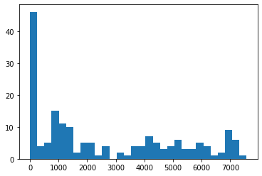
fix missing!!!

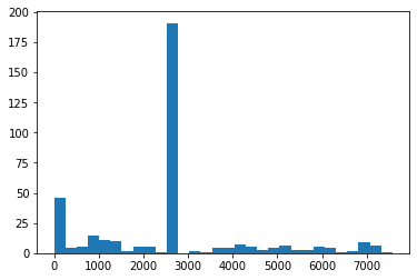
d.Brebeuf.fillna(d.Brebeuf.mean(), inplace=True)

d['Brebeuf'].describe()

count     365.000000
mean     2576.359551
std      1732.161423
min         0.000000
25%      1588.000000
50%      2576.359551
75%      2576.359551
max      7575.000000
Name: Brebeuf, dtype: float64

plt.hist(d.Brebeuf, bins=30);

d

	Berri	Mneuve1	Mneuve2	Brebeuf
Date
2009-01-01	29	20	35	2576.359551
2009-02-01	19	3	22	2576.359551
2009-03-01	24	12	22	2576.359551
2009-04-01	24	8	15	2576.359551
2009-05-01	120	111	141	2576.359551
...	...	...	...	...
2009-12-27	66	29	52	0.000000
2009-12-28	61	41	99	0.000000
2009-12-29	89	52	115	0.000000
2009-12-30	76	43	115	0.000000
2009-12-31	53	46	112	0.000000

365 rows × 4 columns

let’s make sure it is sorted

d.sort_index(inplace=True)
d.head()

	Berri	Mneuve1	Mneuve2	Brebeuf
Date
2009-01-01	29	20	35	2576.359551
2009-01-02	14	2	2	2576.359551
2009-01-03	67	30	80	2576.359551
2009-01-04	0	0	0	2576.359551
2009-01-05	1925	1256	1501	2576.359551

Filtering

d[d.Berri>6000]

	Berri	Mneuve1	Mneuve2	Brebeuf
Date
2009-05-06	6028	4120	4223	2576.359551
2009-06-17	6320	3388	6047	2576.359551
2009-07-15	6100	3767	5536	6939.000000
2009-09-07	6626	4227	5751	7575.000000
2009-10-07	6274	4242	5435	7268.000000

d[(d.Berri>6000) & (d.Brebeuf<7000)]

	Berri	Mneuve1	Mneuve2	Brebeuf
Date
2009-05-06	6028	4120	4223	2576.359551
2009-06-17	6320	3388	6047	2576.359551
2009-07-15	6100	3767	5536	6939.000000

Locating

d[d.Berri>5500].sort_index(axis=0)

	Berri	Mneuve1	Mneuve2	Brebeuf
Date
2009-03-08	5904	3102	4853	7194.000000
2009-05-06	6028	4120	4223	2576.359551
2009-05-08	5611	2646	5201	7121.000000
2009-05-21	5728	3693	5397	2576.359551
2009-06-16	5668	3499	5609	2576.359551
2009-06-17	6320	3388	6047	2576.359551
2009-06-23	5799	3114	5386	2576.359551
2009-07-15	6100	3767	5536	6939.000000
2009-07-20	5607	3825	5092	7064.000000
2009-07-21	5754	3745	5357	6996.000000
2009-07-28	5891	3292	5437	7219.000000
2009-09-07	6626	4227	5751	7575.000000
2009-09-09	5575	2727	6535	6686.000000
2009-10-07	6274	4242	5435	7268.000000
2009-12-08	5538	2368	5107	7127.000000

d.iloc[100:110]

	Berri	Mneuve1	Mneuve2	Brebeuf
Date
2009-04-11	1974	1113	2693	1046.000000
2009-04-12	1108	595	1472	0.000000
2009-04-13	0	0	0	2576.359551
2009-04-14	0	0	0	2576.359551
2009-04-15	0	0	0	2576.359551
2009-04-16	0	0	0	2576.359551
2009-04-17	1286	820	1436	2576.359551
2009-04-18	1178	667	826	2576.359551
2009-04-19	2131	1155	1426	2576.359551
2009-04-20	2709	1697	2646	2576.359551

dates as INDEX have special semantics

d.loc["2009-10-01":"2009-10-10"]

	Berri	Mneuve1	Mneuve2	Brebeuf
Date
2009-10-01	81	45	79	2576.359551
2009-10-02	228	101	260	2576.359551
2009-10-03	366	203	354	2576.359551
2009-10-04	0	0	0	2576.359551
2009-10-05	728	362	523	2576.359551
2009-10-06	3460	2354	3978	2576.359551
2009-10-07	6274	4242	5435	7268.000000
2009-10-08	2999	1545	3185	4187.000000
2009-10-09	5496	2921	6587	6520.000000
2009-10-10	1407	725	1443	1003.000000

can do sorting across any criteria

d.sort_values(by="Berri").head()

	Berri	Mneuve1	Mneuve2	Brebeuf
Date
2009-07-04	0	0	0	2576.359551
2009-03-30	0	0	0	2576.359551
2009-04-04	0	0	0	2576.359551
2009-04-13	0	0	0	2576.359551
2009-04-14	0	0	0	2576.359551

and chain operations

d.sort_values(by="Berri").loc["2009-10-01":"2009-10-10"]

	Berri	Mneuve1	Mneuve2	Brebeuf
Date
2009-10-04	0	0	0	2576.359551
2009-10-01	81	45	79	2576.359551
2009-10-02	228	101	260	2576.359551
2009-10-03	366	203	354	2576.359551
2009-10-05	728	362	523	2576.359551
2009-10-10	1407	725	1443	1003.000000
2009-10-08	2999	1545	3185	4187.000000
2009-10-06	3460	2354	3978	2576.359551
2009-10-09	5496	2921	6587	6520.000000
2009-10-07	6274	4242	5435	7268.000000

Time series operations

d.rolling(3).mean().head(10)

	Berri	Mneuve1	Mneuve2	Brebeuf
Date
2009-01-01	NaN	NaN	NaN	NaN
2009-01-02	NaN	NaN	NaN	NaN
2009-01-03	36.666667	17.333333	39.000000	2576.359551
2009-01-04	27.000000	10.666667	27.333333	2576.359551
2009-01-05	664.000000	428.666667	527.000000	2576.359551
2009-01-06	1733.000000	1116.333333	1409.000000	2576.359551
2009-01-07	3223.333333	1862.666667	2426.000000	2576.359551
2009-01-08	2602.666667	1795.000000	3042.666667	3673.906367
2009-01-09	3277.333333	2029.333333	4055.666667	5128.119850
2009-01-10	2668.000000	1290.333333	4214.666667	4798.666667

d.index = d.index + pd.Timedelta("5m")
d.head()

	Berri	Mneuve1	Mneuve2	Brebeuf
Date
2009-01-01 00:05:00	29	20	35	2576.359551
2009-01-02 00:05:00	14	2	2	2576.359551
2009-01-03 00:05:00	67	30	80	2576.359551
2009-01-04 00:05:00	0	0	0	2576.359551
2009-01-05 00:05:00	1925	1256	1501	2576.359551

d.shift(freq=pd.Timedelta(days=365)).head()

	Berri	Mneuve1	Mneuve2	Brebeuf
Date
2010-01-01 00:05:00	29	20	35	2576.359551
2010-01-02 00:05:00	14	2	2	2576.359551
2010-01-03 00:05:00	67	30	80	2576.359551
2010-01-04 00:05:00	0	0	0	2576.359551
2010-01-05 00:05:00	1925	1256	1501	2576.359551

Downsampling

d.resample(pd.Timedelta("2d")).first().head()

	Berri	Mneuve1	Mneuve2	Brebeuf
Date
2009-01-01	29	20	35	2576.359551
2009-01-03	67	30	80	2576.359551
2009-01-05	1925	1256	1501	2576.359551
2009-01-07	4471	2239	3051	2576.359551
2009-01-09	5298	2796	5765	6939.000000

d.resample(pd.Timedelta("2d")).mean().head()

	Berri	Mneuve1	Mneuve2	Brebeuf
Date
2009-01-01	21.5	11.0	18.5	2576.359551
2009-01-03	33.5	15.0	40.0	2576.359551
2009-01-05	2599.5	1674.5	2113.5	2576.359551
2009-01-07	2267.0	1646.0	3201.0	4222.679775
2009-01-09	3970.5	1409.0	4646.5	4263.500000

Upsampling

d.resample(pd.Timedelta("12h")).first().head()

	Berri	Mneuve1	Mneuve2	Brebeuf
Date
2009-01-01 00:00:00	29.0	20.0	35.0	2576.359551
2009-01-01 12:00:00	NaN	NaN	NaN	NaN
2009-01-02 00:00:00	14.0	2.0	2.0	2576.359551
2009-01-02 12:00:00	NaN	NaN	NaN	NaN
2009-01-03 00:00:00	67.0	30.0	80.0	2576.359551

d.resample(pd.Timedelta("12h")).fillna(method="pad").head()

	Berri	Mneuve1	Mneuve2	Brebeuf
Date
2009-01-01 00:00:00	NaN	NaN	NaN	NaN
2009-01-01 12:00:00	29.0	20.0	35.0	2576.359551
2009-01-02 00:00:00	29.0	20.0	35.0	2576.359551
2009-01-02 12:00:00	14.0	2.0	2.0	2576.359551
2009-01-03 00:00:00	14.0	2.0	2.0	2576.359551

Building Dataframes from other structures

a = np.random.randint(10,size=(20,5))
a

array([[6, 4, 8, 2, 0],
       [8, 9, 7, 4, 9],
       [3, 3, 5, 0, 2],
       [8, 9, 3, 9, 1],
       [6, 9, 4, 5, 9],
       [8, 6, 1, 0, 1],
       [9, 6, 1, 7, 2],
       [0, 7, 4, 6, 1],
       [2, 2, 5, 3, 7],
       [4, 9, 3, 3, 9],
       [7, 3, 5, 6, 8],
       [6, 7, 6, 2, 8],
       [1, 2, 5, 2, 8],
       [6, 7, 6, 9, 4],
       [9, 4, 5, 5, 1],
       [4, 4, 5, 9, 8],
       [4, 4, 1, 1, 2],
       [2, 8, 9, 7, 7],
       [3, 4, 3, 0, 5],
       [5, 8, 5, 6, 2]])

k = pd.DataFrame(a, columns=["uno", "dos", "tres", "cuatro", "cinco"], index=range(10,10+len(a)))
k

	uno	dos	tres	cuatro	cinco
10	6	4	8	2	0
11	8	9	7	4	9
12	3	3	5	0	2
13	8	9	3	9	1
14	6	9	4	5	9
15	8	6	1	0	1
16	9	6	1	7	2
17	0	7	4	6	1
18	2	2	5	3	7
19	4	9	3	3	9
20	7	3	5	6	8
21	6	7	6	2	8
22	1	2	5	2	8
23	6	7	6	9	4
24	9	4	5	5	1
25	4	4	5	9	8
26	4	4	1	1	2
27	2	8	9	7	7
28	3	4	3	0	5
29	5	8	5	6	2

.values access the underlying numpy structure

d.values

array([[2.90000000e+01, 2.00000000e+01, 3.50000000e+01, 2.57635955e+03],
       [1.40000000e+01, 2.00000000e+00, 2.00000000e+00, 2.57635955e+03],
       [6.70000000e+01, 3.00000000e+01, 8.00000000e+01, 2.57635955e+03],
       ...,
       [8.90000000e+01, 5.20000000e+01, 1.15000000e+02, 0.00000000e+00],
       [7.60000000e+01, 4.30000000e+01, 1.15000000e+02, 0.00000000e+00],
       [5.30000000e+01, 4.60000000e+01, 1.12000000e+02, 0.00000000e+00]])

some out-of-the-box plotting

but recall that we always can do custom plotting

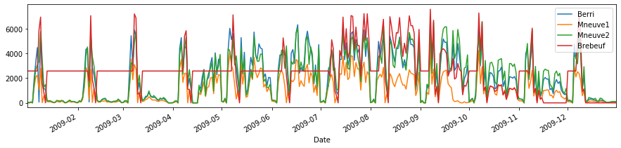
d.plot(figsize=(15,3))

<matplotlib.axes._subplots.AxesSubplot at 0x7fb9f2a9ac10>

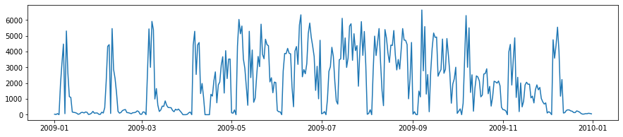
plt.figure(figsize=(15,3))
plt.plot(d.Berri)

[<matplotlib.lines.Line2D at 0x7fb9f29f2250>]

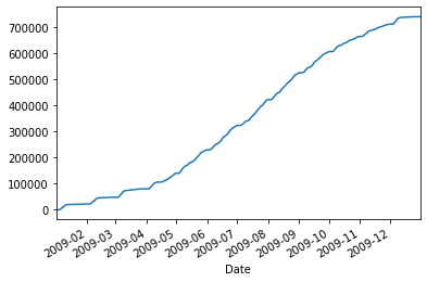
d.Berri.cumsum().plot()

<matplotlib.axes._subplots.AxesSubplot at 0x7fb9f294c450>

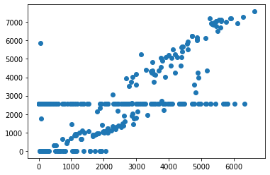
plt.scatter(d.Berri, d.Brebeuf)

<matplotlib.collections.PathCollection at 0x7fb9f360fb50>

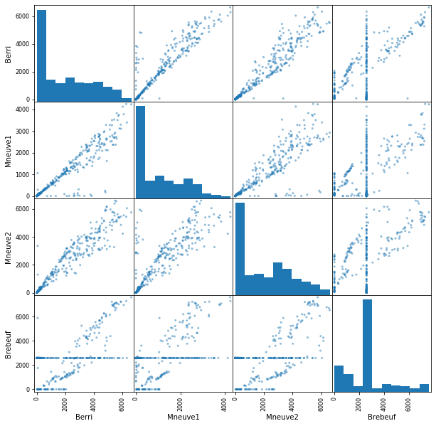
pd.plotting.scatter_matrix(d, figsize=(10,10));

Grouping

d["month"] = [i.month for i in d.index]
d.head()

	Berri	Mneuve1	Mneuve2	Brebeuf	month
Date
2009-01-01 00:05:00	29	20	35	2576.359551	1
2009-01-02 00:05:00	14	2	2	2576.359551	1
2009-01-03 00:05:00	67	30	80	2576.359551	1
2009-01-04 00:05:00	0	0	0	2576.359551	1
2009-01-05 00:05:00	1925	1256	1501	2576.359551	1

d.groupby("month").max()

	Berri	Mneuve1	Mneuve2	Brebeuf
month
1	5298	2796	5765	6939.0
2	5451	2868	5517	7052.0
3	5904	3523	5762	7194.0
4	5278	3499	5327	5837.0
5	6028	4120	5397	7121.0
6	6320	3499	6047	5259.0
7	6100	3825	5536	7219.0
8	5452	2865	6379	7044.0
9	6626	4227	6535	7575.0
10	6274	4242	6587	7268.0
11	4864	2648	5895	6044.0
12	5538	2983	5107	7127.0

d.groupby("month").count()

	Berri	Mneuve1	Mneuve2	Brebeuf
month
1	31	31	31	31
2	28	28	28	28
3	31	31	31	31
4	30	30	30	30
5	31	31	31	31
6	30	30	30	30
7	31	31	31	31
8	31	31	31	31
9	30	30	30	30
10	31	31	31	31
11	30	30	30	30
12	31	31	31	31

Time series

observe we can establish at load time many thing if the dataset is relatively clean

tiempo=pd.read_csv('local/data/weather_data_austin_2010.csv',parse_dates=['Date'], dayfirst=True ,index_col='Date')
tiempo

	Temperature	DewPoint	Pressure
Date
2010-01-01 00:00:00	46.2	37.5	1.0
2010-01-01 01:00:00	44.6	37.1	1.0
2010-01-01 02:00:00	44.1	36.9	1.0
2010-01-01 03:00:00	43.8	36.9	1.0
2010-01-01 04:00:00	43.5	36.8	1.0
...	...	...	...
2010-12-31 19:00:00	51.1	38.1	1.0
2010-12-31 20:00:00	49.0	37.9	1.0
2010-12-31 21:00:00	47.9	37.9	1.0
2010-12-31 22:00:00	46.9	37.9	1.0
2010-12-31 23:00:00	46.2	37.7	1.0

8759 rows × 3 columns

tiempo.loc['2010-08-01':'2010-10-30']

	Temperature	DewPoint	Pressure
Date
2010-08-01 00:00:00	79.0	70.8	1.0
2010-08-01 01:00:00	77.4	71.2	1.0
2010-08-01 02:00:00	76.4	71.3	1.0
2010-08-01 03:00:00	75.7	71.4	1.0
2010-08-01 04:00:00	75.1	71.4	1.0
...	...	...	...
2010-10-30 19:00:00	65.4	53.6	1.0
2010-10-30 20:00:00	63.6	53.9	1.0
2010-10-30 21:00:00	62.2	53.8	1.0
2010-10-30 22:00:00	61.4	54.0	1.0
2010-10-30 23:00:00	60.3	53.9	1.0

2184 rows × 3 columns

tiempo.loc['2010-06'].head()

	Temperature	DewPoint	Pressure
Date
2010-06-01 00:00:00	74.0	67.9	1.0
2010-06-01 01:00:00	72.6	68.0	1.0
2010-06-01 02:00:00	72.0	67.9	1.0
2010-06-01 03:00:00	71.6	67.9	1.0
2010-06-01 04:00:00	71.1	67.7	1.0

tiempo.sample(10)

	Temperature	DewPoint	Pressure
Date
2010-12-24 20:00:00	48.9	38.6	1.0
2010-10-12 01:00:00	64.7	59.3	1.0
2010-02-21 03:00:00	49.3	42.8	1.0
2010-07-20 16:00:00	93.5	67.1	1.0
2010-11-04 12:00:00	70.4	53.0	1.0
2010-10-29 15:00:00	75.4	53.0	1.0
2010-07-18 17:00:00	92.5	67.3	1.0
2010-04-16 13:00:00	76.4	56.7	1.0
2010-07-05 06:00:00	74.4	71.2	1.0
2010-07-03 16:00:00	91.4	68.6	1.0

tiempo.sample(frac=0.01)

	Temperature	DewPoint	Pressure
Date
2010-12-22 23:00:00	45.9	37.8	1.0
2010-05-19 15:00:00	84.9	64.8	1.0
2010-02-24 12:00:00	61.9	44.5	1.0
2010-01-10 00:00:00	46.2	37.4	1.0
2010-12-21 19:00:00	50.7	38.8	1.0
...	...	...	...
2010-05-27 11:00:00	81.7	67.3	1.0
2010-08-11 03:00:00	75.8	71.3	1.0
2010-03-17 13:00:00	68.5	49.6	1.0
2010-10-28 14:00:00	75.2	53.9	1.0
2010-08-21 03:00:00	75.9	71.1	1.0

88 rows × 3 columns

Resampling

tiempo.head()

	Temperature	DewPoint	Pressure
Date
2010-01-01 00:00:00	46.2	37.5	1.0
2010-01-01 01:00:00	44.6	37.1	1.0
2010-01-01 02:00:00	44.1	36.9	1.0
2010-01-01 03:00:00	43.8	36.9	1.0
2010-01-01 04:00:00	43.5	36.8	1.0

tiempo.resample("5d").mean().head()

	Temperature	DewPoint	Pressure
Date
2010-01-01	49.720833	38.092500	1.0
2010-01-06	49.449167	37.575000	1.0
2010-01-11	49.222500	37.603333	1.0
2010-01-16	49.441667	37.650000	1.0
2010-01-21	50.683333	39.309167	1.0

tiempo.resample("5d").mean().head()

	Temperature	DewPoint	Pressure
Date
2010-01-01	49.720833	38.092500	1.0
2010-01-06	49.449167	37.575000	1.0
2010-01-11	49.222500	37.603333	1.0
2010-01-16	49.441667	37.650000	1.0
2010-01-21	50.683333	39.309167	1.0

tiempo.resample("5d").mean().head()

	Temperature	DewPoint	Pressure
Date
2010-01-01	49.720833	38.092500	1.0
2010-01-06	49.449167	37.575000	1.0
2010-01-11	49.222500	37.603333	1.0
2010-01-16	49.441667	37.650000	1.0
2010-01-21	50.683333	39.309167	1.0

tiempo.resample("30min").mean()[:15]

	Temperature	DewPoint	Pressure
Date
2010-01-01 00:00:00	46.2	37.5	1.0
2010-01-01 00:30:00	NaN	NaN	NaN
2010-01-01 01:00:00	44.6	37.1	1.0
2010-01-01 01:30:00	NaN	NaN	NaN
2010-01-01 02:00:00	44.1	36.9	1.0
2010-01-01 02:30:00	NaN	NaN	NaN
2010-01-01 03:00:00	43.8	36.9	1.0
2010-01-01 03:30:00	NaN	NaN	NaN
2010-01-01 04:00:00	43.5	36.8	1.0
2010-01-01 04:30:00	NaN	NaN	NaN
2010-01-01 05:00:00	43.0	36.5	1.0
2010-01-01 05:30:00	NaN	NaN	NaN
2010-01-01 06:00:00	43.1	36.3	1.0
2010-01-01 06:30:00	NaN	NaN	NaN
2010-01-01 07:00:00	42.3	35.9	1.0

subt=tiempo.between_time(start_time='1:00',end_time='12:00')
subt

	Temperature	DewPoint	Pressure
Date
2010-01-01 01:00:00	44.6	37.1	1.0
2010-01-01 02:00:00	44.1	36.9	1.0
2010-01-01 03:00:00	43.8	36.9	1.0
2010-01-01 04:00:00	43.5	36.8	1.0
2010-01-01 05:00:00	43.0	36.5	1.0
...	...	...	...
2010-12-31 08:00:00	42.5	36.1	1.0
2010-12-31 09:00:00	46.0	37.7	1.0
2010-12-31 10:00:00	49.4	38.0	1.0
2010-12-31 11:00:00	52.4	38.0	1.0
2010-12-31 12:00:00	54.7	37.9	1.0

4379 rows × 3 columns

tiempo.index.weekday

Int64Index([4, 4, 4, 4, 4, 4, 4, 4, 4, 4,
            ...
            4, 4, 4, 4, 4, 4, 4, 4, 4, 4],
           dtype='int64', name='Date', length=8759)

tiempo.index.month

Int64Index([ 1,  1,  1,  1,  1,  1,  1,  1,  1,  1,
            ...
            12, 12, 12, 12, 12, 12, 12, 12, 12, 12],
           dtype='int64', name='Date', length=8759)

tiempo.index.day

Int64Index([ 1,  1,  1,  1,  1,  1,  1,  1,  1,  1,
            ...
            31, 31, 31, 31, 31, 31, 31, 31, 31, 31],
           dtype='int64', name='Date', length=8759)

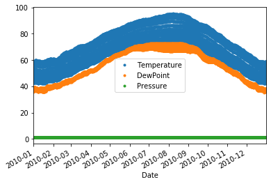
tiempo.plot(style='.')

<matplotlib.axes._subplots.AxesSubplot at 0x7fb9e70c8250>

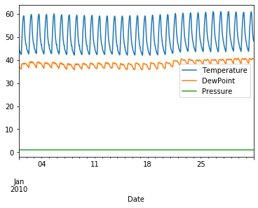
tiempo['2010-01'].plot()

<matplotlib.axes._subplots.AxesSubplot at 0x7fb9f2af66d0>

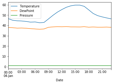
tiempo['2010-01-04'].plot()

<matplotlib.axes._subplots.AxesSubplot at 0x7fb9f2b8eed0>

Rolling operations

import pandas as pd
### permite obtener data frames directamente de internet
!pip install yfinance

Collecting yfinance
  Downloading https://files.pythonhosted.org/packages/c2/31/8b374a12b90def92a4e27d0fc595fc43635f395984e36a075244d98bd265/yfinance-0.1.54.tar.gz
Collecting pandas>=0.24
?25l  Downloading https://files.pythonhosted.org/packages/4a/6a/94b219b8ea0f2d580169e85ed1edc0163743f55aaeca8a44c2e8fc1e344e/pandas-1.0.3-cp37-cp37m-manylinux1_x86_64.whl (10.0MB)
     |████████████████████████████████| 10.0MB 453kB/s eta 0:00:01
?25hRequirement already satisfied: numpy>=1.15 in /opt/anaconda3/lib/python3.7/site-packages (from yfinance) (1.15.1)
Requirement already satisfied: requests>=2.20 in /opt/anaconda3/lib/python3.7/site-packages (from yfinance) (2.22.0)
Collecting multitasking>=0.0.7
  Downloading https://files.pythonhosted.org/packages/69/e7/e9f1661c28f7b87abfa08cb0e8f51dad2240a9f4f741f02ea839835e6d18/multitasking-0.0.9.tar.gz
Requirement already satisfied: pytz>=2017.2 in /opt/anaconda3/lib/python3.7/site-packages (from pandas>=0.24->yfinance) (2018.5)
Requirement already satisfied: python-dateutil>=2.6.1 in /opt/anaconda3/lib/python3.7/site-packages (from pandas>=0.24->yfinance) (2.7.3)
Requirement already satisfied: idna<2.9,>=2.5 in /opt/anaconda3/lib/python3.7/site-packages (from requests>=2.20->yfinance) (2.8)
Requirement already satisfied: certifi>=2017.4.17 in /opt/anaconda3/lib/python3.7/site-packages (from requests>=2.20->yfinance) (2019.9.11)
Requirement already satisfied: chardet<3.1.0,>=3.0.2 in /opt/anaconda3/lib/python3.7/site-packages (from requests>=2.20->yfinance) (3.0.4)
Requirement already satisfied: urllib3!=1.25.0,!=1.25.1,<1.26,>=1.21.1 in /opt/anaconda3/lib/python3.7/site-packages (from requests>=2.20->yfinance) (1.24.2)
Requirement already satisfied: six>=1.5 in /opt/anaconda3/lib/python3.7/site-packages (from python-dateutil>=2.6.1->pandas>=0.24->yfinance) (1.13.0)
Building wheels for collected packages: yfinance, multitasking
  Building wheel for yfinance (setup.py) ... ?25ldone
?25h  Created wheel for yfinance: filename=yfinance-0.1.54-py2.py3-none-any.whl size=22411 sha256=d937a7a089b0883844df4d4f388c8bcc4dc145446c43e698a5181e6ebd099621
  Stored in directory: /home/rlx/.cache/pip/wheels/f9/e3/5b/ec24dd2984b12d61e0abf26289746c2436a0e7844f26f2515c
  Building wheel for multitasking (setup.py) ... ?25ldone
?25h  Created wheel for multitasking: filename=multitasking-0.0.9-cp37-none-any.whl size=8368 sha256=bfe866419b7d2ac5e39bab8a20d2378ac727b56d6dc6e3f248e2a4115ea368bb
  Stored in directory: /home/rlx/.cache/pip/wheels/37/fa/73/d492849e319038eb4d986f5152e4b19ffb1bc0639da84d2677
Successfully built yfinance multitasking
Installing collected packages: pandas, multitasking, yfinance
  Found existing installation: pandas 0.23.4
    Uninstalling pandas-0.23.4:
      Successfully uninstalled pandas-0.23.4
Successfully installed multitasking-0.0.9 pandas-1.0.3 yfinance-0.1.54

import yfinance as yf

#define the ticker symbol
tickerSymbol = 'MSFT'

#get data on this ticker
tickerData = yf.Ticker(tickerSymbol)

#get the historical prices for this ticker
gs = tickerData.history(period='1d', start='2010-1-1', end='2020-1-25')

#see your data
gs

	Open	High	Low	Close	Volume	Dividends	Stock Splits
Date
2010-01-04	24.04	24.41	24.01	24.29	38409100	0.0	0
2010-01-05	24.22	24.41	24.05	24.30	49749600	0.0	0
2010-01-06	24.24	24.40	23.96	24.15	58182400	0.0	0
2010-01-07	24.04	24.10	23.70	23.90	50559700	0.0	0
2010-01-08	23.77	24.24	23.74	24.07	51197400	0.0	0
...	...	...	...	...	...	...	...
2020-01-17	166.96	167.01	164.98	166.64	34371700	0.0	0
2020-01-21	166.23	167.73	165.98	166.05	29517200	0.0	0
2020-01-22	166.94	167.03	165.23	165.25	24138800	0.0	0
2020-01-23	165.74	166.35	164.82	166.27	19680800	0.0	0
2020-01-24	167.05	167.07	164.00	164.59	24918100	0.0	0

2532 rows × 7 columns

gs.Close.rolling(10).mean().head(20)

Date
2010-01-04       NaN
2010-01-05       NaN
2010-01-06       NaN
2010-01-07       NaN
2010-01-08       NaN
2010-01-11       NaN
2010-01-12       NaN
2010-01-13       NaN
2010-01-14       NaN
2010-01-15    24.041
2010-01-19    24.053
2010-01-20    24.024
2010-01-21    23.965
2010-01-22    23.848
2010-01-25    23.742
2010-01-26    23.682
2010-01-27    23.651
2010-01-28    23.558
2010-01-29    23.340
2010-02-01    23.148
Name: Close, dtype: float64

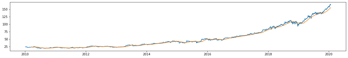
plt.figure(figsize=(20,3))
plt.plot(gs.Close)
plt.plot(gs.Close.rolling(50).mean())

[<matplotlib.lines.Line2D at 0x7fb9f289bc90>]

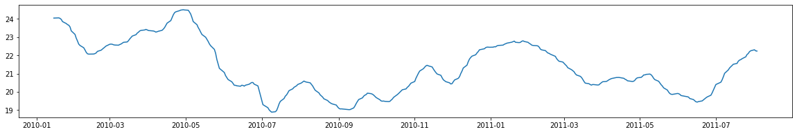
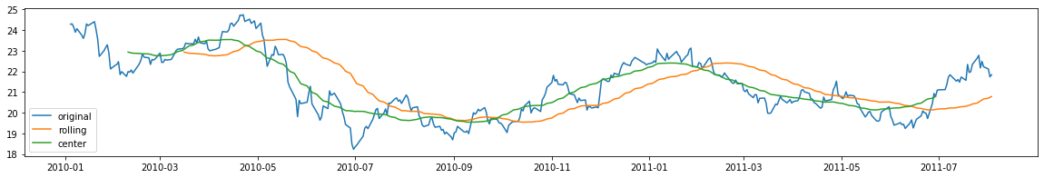
plt.figure(figsize=(20,3))
plt.plot(gs.iloc[:400].Close, label="original")
plt.plot(gs.iloc[:400].Close.rolling(50).mean(), label="rolling")
plt.plot(gs.iloc[:400].Close.rolling(50, center=True).mean(), label="center")
plt.legend();

plt.figure(figsize=(20,3))
plt.plot(gs.iloc[:400].Close.rolling(10).mean())

[<matplotlib.lines.Line2D at 0x7fb9f26eff50>]