
04.03 - HYPOTHESIS TESTING#
!wget --no-cache -O init.py -q https://raw.githubusercontent.com/rramosp/ai4eng.v1/main/content/init.py
import init; init.init(force_download=False); init.get_weblink()
endpoint https://m5knaekxo6.execute-api.us-west-2.amazonaws.com/dev-v0001/rlxmooc
from scipy import stats
import numpy as np
import matplotlib.pyplot as plt
from progressbar import progressbar as pbar
%matplotlib inline
Stochastic models#
A probabilistic (or stochastic) model is one that assigns probabilities to the different objects or events it attempts to describe. For instance,
The probability of a patient to have different glucose levels.
The probability of students to obtain different scores in an exam
A stochastic model
Just provides a probability for each object (a number between 0 and 1)
Does not necessarily provide an explanation on HOW probabilities arise.
Is given as a probability distribution with its corresponding PDF (probability density function), by which we can compute any probability
Confidence on models#
STEP 1: Define the model you want to challenge (the NULL Hypothesis \(H_0\))#
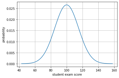
A researcher brings a stochastic model claiming that students’ scores in a certain exam follow a normal distribution with \(\mu=100\) and \(\sigma=15\).
h0 = stats.norm(loc=100, scale=15)
x = h0.rvs(10000)
rx = np.linspace(np.min(x), np.max(x), 100)
plt.plot(rx, h0.pdf(rx))
plt.grid(); plt.xlabel("student exam score"); plt.ylabel("probability")
Text(0, 0.5, 'probability')
You are NOT SURE if the model works well with your students, so you start looking (sampling) at their exam scores. How much would you trust the model in the following cases:
H1: You sample 5 students and their average score is 110
H2: You sample 5 students and their average score is 105
H3: You sample 30 students and their average score is 105
STEP 2: Define your REAL WORLD sample and your test statistic#
The test statistic is what you are interesting in computing from a real world sample.
SAMPLE: a set of 5 students.
TEST STATISTIC: the average exam score of the sample
STEP 3: Understand the TEST STATISTIC distribution under \(H_0\) (if the model is True)#
We will NOT USE FORMULAS, only SIMULATION#
Let’s assume the model is right, let’s SIMULATE we select 5 students from the model’s probability distribution. We do 10 simulations.
Run the cells below several times, and ask yourself the following questions:
how probable is that you see 5 students with average score 110 or higher?
how probable is that you see 5 students with average score 105 or higher?
m = stats.norm(loc=100, scale=15)
for n in range(20):
    s = m.rvs(5)
    print ("sample %2d: "%n+ " ".join(["%5.1f"%i for i in s]), " mean: %7.2f"%np.mean(s))
sample  0:  80.5 119.2 105.4  95.7 104.8  mean:  101.11
sample  1: 111.8  94.3  99.3  76.9  99.4  mean:   96.34
sample  2: 105.2  91.0 103.9  89.7 105.3  mean:   99.01
sample  3: 113.5 123.8 107.7 108.4  86.6  mean:  108.00
sample  4: 100.2 108.6  90.2 102.3  97.2  mean:   99.67
sample  5:  72.8  81.4 109.3  76.9 129.1  mean:   93.92
sample  6: 106.9  73.1 115.9  92.0  84.5  mean:   94.48
sample  7:  76.8 105.7  95.3  99.7  83.0  mean:   92.10
sample  8:  95.8 112.8 129.0  98.8  86.6  mean:  104.61
sample  9:  93.1  99.3  91.2  83.9  81.5  mean:   89.80
sample 10: 102.9  78.2  69.1  97.6 114.8  mean:   92.50
sample 11:  92.0 108.9  91.9  91.7  83.2  mean:   93.56
sample 12:  99.0 114.0 102.5 121.7  93.2  mean:  106.07
sample 13: 104.9  65.4 112.6 103.8  99.6  mean:   97.27
sample 14: 121.3 100.0 117.9  97.5 110.2  mean:  109.39
sample 15: 111.2  88.0 104.6  95.9  70.2  mean:   93.99
sample 16: 106.2  99.8 103.4 113.7 109.2  mean:  106.47
sample 17:  96.3  87.0 106.6 114.0 108.8  mean:  102.56
sample 18: 115.1  86.9 109.0  84.7 115.4  mean:  102.21
sample 19:  95.0 109.6 110.1 115.6 116.4  mean:  109.36
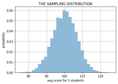
let’s do the simulation 10000 times and answer the questions
z = np.r_[[np.mean(m.rvs(5)) for _ in range(10000)]]

plt.hist(z, bins=30, density=True, alpha=.5);
plt.grid(); plt.xlabel("avg score for 5 students"); plt.ylabel("probability")
plt.title("THE SAMPLING DISTRIBUTION"); plt.show()
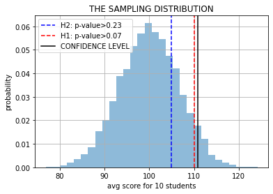
STEP 4: measure the likelihood of the REAL WORLD sample w.r.t. \(H_0\)#
let’s see and measure where our REAL WORLD sample falls in the distribution for the test statistic under \(H_0\)
if our REAL WORLD sample is too rare \(\rightarrow\) we have less trust in the \(H_0\) model
if our REAL WORLD sample is common \(\rightarrow\) we have more trust in the \(H_0\) model
z = np.r_[[np.mean(m.rvs(5)) for _ in range(10000)]]

plt.hist(z, bins=30, density=True, alpha=.5);
plt.axvline(105, color="blue", ls="--", label="H2: p-value>%.2f"%np.mean(z>105))
plt.axvline(110, color="red", ls="--", label="H1: p-value>%.2f"%np.mean(z>110))
plt.axvline(np.percentile(z, 95), color="black", label="CONFIDENCE LEVEL")
plt.grid(); plt.xlabel("avg score for 10 students"); plt.ylabel("probability")
plt.legend(); plt.title("THE SAMPLING DISTRIBUTION"); plt.show()
Now, if when we took 5 students we measured an average score of 115 or 105, would you trust this model?
Observe that,
We only have ONE REAL WORLD SAMPLE, but we made 10000 SIMULATIONS.
The distribution above is called the SAMPLING DISTRIBUTION.
The p-value is the probability of seeing something like our REAL WORLD SAMPLE, or even more extreme, according to the model we are testing.
What we did is called a Z-TEST.
It is standard to consider a p-value<0.05 to indicate that our REAL WORLD SAMPLE has a very small probability according to the model and thus, there must be something wrong with the model.
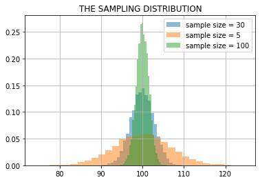
Central Limit Theorem: regardless the shape of the original disitrution, the sampling distribution will always be a Normal distribution.
Challenge: understand the Python code for sampling
What if we consider H3, with 30 students?#
Another simulation, another sampling distribution.
z = np.r_[[np.mean(m.rvs(30)) for _ in range(10000)]]

plt.hist(z, bins=30, density=True, alpha=.5);
plt.axvline(105, color="blue", ls="--",  label="H2: p-value>%.2f"%np.mean(z>105))
plt.grid(); plt.xlabel("avg score for 30 students"); plt.ylabel("probability")
plt.axvline(np.percentile(z, 95), color="black", label="CONFIDENCE LEVEL")
plt.legend(); plt.title("THE SAMPLING DISTRIBUTION"); plt.show()
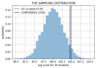
WE HAVE LEST TRUST IN OUR MODEL NOW!! \(\rightarrow\) WHY?
z1 = np.r_[[np.mean(m.rvs(30)) for _ in range(10000)]]
z2 = np.r_[[np.mean(m.rvs(5)) for _ in range(10000)]]
z3 = np.r_[[np.mean(m.rvs(100)) for _ in range(10000)]]

plt.hist(z1, bins=30, density=True, alpha=.5, label="sample size = 30");
plt.hist(z2, bins=30, density=True, alpha=.5, label="sample size = 5");
plt.hist(z3, bins=30, density=True, alpha=.5, label="sample size = 100");
plt.grid(); plt.legend(); plt.title("THE SAMPLING DISTRIBUTION"); plt.show()
plt.show();
Terminology#
NULL HYPOTHESIS \(H_0\): The model we are testing whether we can reject it or not.
REAL WORLD SAMPLE: What we measure in reality to a limited number of objects.
TEST STATISTIC: What we compute from the real world sample (the average, in our case).
SAMPLING DISTRIBUTION: The distribution of simulating many real world examples and computing the test statistic to each of them.
p-value: The probability of seeing in the simulation something as rare as our real world example.
CONFIDENCE LEVEL: The minimum p-value we are willing to observe to NOT consider to distrust \(H_0\)
REJECT \(H_0\): When we observe a p-value lower than the confidence level, meaning that our real world sample is too rare.
FAIL TO REJECT \(H_0\): When we observe a p-value higher than the confidence level, meaning that our real world sample is fairly normal.
MONTE CARLO SIMULATION: What we did!!!
Simulations and Formulas#
We do simulation because we have computers. When these tests were invented, computers were not around, so people developed tables and formulas to compute by hand the p-values.
If simulating is hard we can always use the analytical formula.
Where \(\mathcal{N}(0,1).\text{cdf}\) is the Cummulative Density Function of the Standard Normal distribution
real_world_sample_mean = 105
real_world_sample_size = 5
model_mu = 100
model_sigma = 15
z = np.r_[[np.mean(m.rvs(real_world_sample_size)) for _ in range(10000)]]
print ("simulated p-value %.3f"%np.mean(real_world_sample_mean<z))
simulated p-value 0.238
print ("analytical, p-value %.3f"%(1-stats.norm().cdf((real_world_sample_mean-model_mu)\
                                                    /(model_sigma/np.sqrt(real_world_sample_size)))))
analytical, p-value 0.228
For more info:
Sampling distribution of the sample mean Khan Academy
Central limit theorem Wikipedia