05.03 - MODEL SELECTION

!wget --no-cache -O init.py -q https://raw.githubusercontent.com/rramosp/ai4eng.v1/main/content/init.py
import init; init.init(force_download=False); init.get_weblink()

import numpy as np
import matplotlib.pyplot as plt
import pandas as pd
import local.lib.timeseries as ts
%matplotlib inline

RULE: we cannot use the same data to BOTH make choices on our precessing pipeline AND report performance

dataset = pd.read_csv("local/data/cal_housing.data")
dataset = dataset.sample(len(dataset))

d = dataset.iloc[:10000].sample(1000)
X = d.values[:,:-1]
y = d["medianHouseValue"].values
print (X.shape, y.shape)

(1000, 5) (1000,)

from sklearn.linear_model import LinearRegression
from sklearn.svm import SVR
from sklearn.ensemble import RandomForestRegressor
from sklearn.tree import DecisionTreeRegressor
from sklearn.model_selection import train_test_split
from sklearn.metrics import median_absolute_error, r2_score, mean_squared_error

def rel_mrae(estimator, X, y):
    preds = estimator.predict(X)
    return np.mean(np.abs(preds-y)/y)

Let’s consider we are choosing between different models with any crossval technique

We start by using a regular train/test split with resampling

from sklearn.model_selection import cross_validate, ShuffleSplit

MODEL 1

estimator1 = DecisionTreeRegressor(max_depth=5)
z1 = cross_validate(estimator1, X, y, return_train_score=True, return_estimator=True,
                    scoring=rel_mrae, cv=ShuffleSplit(n_splits=10, test_size=0.1))

z1

{'fit_time': array([0.0026865 , 0.00383544, 0.0037663 , 0.00304556, 0.00305915,
        0.00277185, 0.00263572, 0.00275302, 0.00315762, 0.00289965]),
 'score_time': array([0.00101566, 0.00098491, 0.00112557, 0.00090575, 0.00094485,
        0.00083876, 0.00069666, 0.00081682, 0.00074935, 0.00079894]),
 'estimator': (DecisionTreeRegressor(ccp_alpha=0.0, criterion='mse', max_depth=5,
                        max_features=None, max_leaf_nodes=None,
                        min_impurity_decrease=0.0, min_impurity_split=None,
                        min_samples_leaf=1, min_samples_split=2,
                        min_weight_fraction_leaf=0.0, presort='deprecated',
                        random_state=None, splitter='best'),
  DecisionTreeRegressor(ccp_alpha=0.0, criterion='mse', max_depth=5,
                        max_features=None, max_leaf_nodes=None,
                        min_impurity_decrease=0.0, min_impurity_split=None,
                        min_samples_leaf=1, min_samples_split=2,
                        min_weight_fraction_leaf=0.0, presort='deprecated',
                        random_state=None, splitter='best'),
  DecisionTreeRegressor(ccp_alpha=0.0, criterion='mse', max_depth=5,
                        max_features=None, max_leaf_nodes=None,
                        min_impurity_decrease=0.0, min_impurity_split=None,
                        min_samples_leaf=1, min_samples_split=2,
                        min_weight_fraction_leaf=0.0, presort='deprecated',
                        random_state=None, splitter='best'),
  DecisionTreeRegressor(ccp_alpha=0.0, criterion='mse', max_depth=5,
                        max_features=None, max_leaf_nodes=None,
                        min_impurity_decrease=0.0, min_impurity_split=None,
                        min_samples_leaf=1, min_samples_split=2,
                        min_weight_fraction_leaf=0.0, presort='deprecated',
                        random_state=None, splitter='best'),
  DecisionTreeRegressor(ccp_alpha=0.0, criterion='mse', max_depth=5,
                        max_features=None, max_leaf_nodes=None,
                        min_impurity_decrease=0.0, min_impurity_split=None,
                        min_samples_leaf=1, min_samples_split=2,
                        min_weight_fraction_leaf=0.0, presort='deprecated',
                        random_state=None, splitter='best'),
  DecisionTreeRegressor(ccp_alpha=0.0, criterion='mse', max_depth=5,
                        max_features=None, max_leaf_nodes=None,
                        min_impurity_decrease=0.0, min_impurity_split=None,
                        min_samples_leaf=1, min_samples_split=2,
                        min_weight_fraction_leaf=0.0, presort='deprecated',
                        random_state=None, splitter='best'),
  DecisionTreeRegressor(ccp_alpha=0.0, criterion='mse', max_depth=5,
                        max_features=None, max_leaf_nodes=None,
                        min_impurity_decrease=0.0, min_impurity_split=None,
                        min_samples_leaf=1, min_samples_split=2,
                        min_weight_fraction_leaf=0.0, presort='deprecated',
                        random_state=None, splitter='best'),
  DecisionTreeRegressor(ccp_alpha=0.0, criterion='mse', max_depth=5,
                        max_features=None, max_leaf_nodes=None,
                        min_impurity_decrease=0.0, min_impurity_split=None,
                        min_samples_leaf=1, min_samples_split=2,
                        min_weight_fraction_leaf=0.0, presort='deprecated',
                        random_state=None, splitter='best'),
  DecisionTreeRegressor(ccp_alpha=0.0, criterion='mse', max_depth=5,
                        max_features=None, max_leaf_nodes=None,
                        min_impurity_decrease=0.0, min_impurity_split=None,
                        min_samples_leaf=1, min_samples_split=2,
                        min_weight_fraction_leaf=0.0, presort='deprecated',
                        random_state=None, splitter='best'),
  DecisionTreeRegressor(ccp_alpha=0.0, criterion='mse', max_depth=5,
                        max_features=None, max_leaf_nodes=None,
                        min_impurity_decrease=0.0, min_impurity_split=None,
                        min_samples_leaf=1, min_samples_split=2,
                        min_weight_fraction_leaf=0.0, presort='deprecated',
                        random_state=None, splitter='best')),
 'test_score': array([0.37247763, 0.40161065, 0.42150456, 0.47736097, 0.42858179,
        0.36527219, 0.38721038, 0.34214222, 0.31086012, 0.33274428]),
 'train_score': array([0.34318495, 0.32977355, 0.32523023, 0.33635713, 0.32606125,
        0.32962278, 0.34875038, 0.34060793, 0.3374607 , 0.34459654])}

def report_cv_score(z):
    print ("test score   %.3f (±%.4f) with %d splits"%(np.mean(z["test_score"]), np.std(z["test_score"]), len(z["test_score"])))
    print ("train score  %.3f (±%.4f) with %d splits"%(np.mean(z["train_score"]), np.std(z["train_score"]), len(z["train_score"])))
    
report_cv_score(z1)    

test score   0.384 (±0.0476) with 10 splits
train score  0.336 (±0.0078) with 10 splits

MODEL 2

from sklearn.ensemble import RandomForestRegressor
estimator2 = DecisionTreeRegressor(max_depth=10)
z2 = cross_validate(estimator2, X, y, return_train_score=True, return_estimator=True,
                    scoring=rel_mrae, cv=ShuffleSplit(n_splits=10, test_size=0.1))  
report_cv_score(z2)    

test score   0.367 (±0.0383) with 10 splits
train score  0.111 (±0.0113) with 10 splits

MODEL 3

from sklearn.linear_model import LinearRegression
estimator3 = LinearRegression()
z3 = cross_validate(estimator3, X, y, return_train_score=True, return_estimator=True,
                    scoring=rel_mrae, cv=ShuffleSplit(n_splits=10, test_size=0.1))
report_cv_score(z3)

test score   0.455 (±0.0233) with 10 splits
train score  0.431 (±0.0060) with 10 splits

Some questions:

• what would be our model of choice: probably estimator2. CORRECT

• what is the performance associated with our choice: the test score reported by estimator2. INCORRECT

• we need to physically deliver our trained model to the appropriate business area, but we trained several models for statistical stability. Which model shall we hand over?

we cannot use the same data to make a choice AND report a result.

observe the performance measured with the models we trained before on new production data

ed = dataset[10000:].sample(1000)
eX = ed.values[:,:-1]
ey = ed["medianHouseValue"].values
print (eX.shape, ey.shape)

(1000, 5) (1000,)

scores = [rel_mrae(estimator, eX, ey) for estimator in z2["estimator"]]
print ("scores", scores)
print ("mean score %.3f (±%.4f) with %d splits"%(np.mean(scores), np.std(scores), len(scores)))

scores [0.34704496772017795, 0.35181627445650004, 0.3780380631512966, 0.3473043719704006, 0.3303955214044563, 0.4078152917670846, 0.3454037329742688, 0.34298337274978824, 0.3505249600341739, 0.3482397402889321]
mean score 0.355 (±0.0209) with 10 splits

use train/val/test splits

• use train/val to train and select model

• use test split ONLY to measure performance of the selected model

literature and resources use test/val interchangeably, or sometimes dev instead of val

observe how we:

• do a first split with 10% for test and 90% for train/val

• adjust val size so that when selecting x% of 90% train/val, ends up having the same number of elements as in test

from sklearn.model_selection import train_test_split

test_size = 0.3
number_of_houses_for_trainval = 1000

val_size  = test_size/(1-test_size) # so that the have the same number of elements

assert number_of_houses_for_trainval<10000, "too many houses for trainval"


d = dataset.iloc[:10000].sample(number_of_houses_for_trainval)
X = d.values[:,:-1]
y = d["medianHouseValue"].values
print (X.shape, y.shape)

print ("test size %.2f"%test_size)
print ("val size is %.2f (relative to %.2f) "%(val_size, 1-test_size))

Xtv, Xts, ytv, yts = train_test_split(X, y, test_size=test_size)
print (Xtv.shape, Xts.shape)

(1000, 5) (1000,)
test size 0.30
val size is 0.43 (relative to 0.70) 
(700, 5) (300, 5)

PART 1: we AUTOMATE the model selection process

zscores = []
estimators = [estimator1, estimator2, estimator3]
for estimator in estimators:
    print("--")
    z = cross_validate(estimator, Xtv, ytv, return_train_score=True, return_estimator=False,
                       scoring=rel_mrae, cv=ShuffleSplit(n_splits=10, test_size=val_size))
    report_cv_score(z)
    zscores.append(np.mean(z["test_score"]))
best = np.argmin(zscores)
print ("selecting ", best)
best_estimator = estimators[best]
print ("\nselected model")
print (best_estimator)

--
test score   0.473 (±0.0475) with 10 splits
train score  0.347 (±0.0423) with 10 splits
--
test score   0.416 (±0.0335) with 10 splits
train score  0.092 (±0.0213) with 10 splits
--
test score   0.486 (±0.0305) with 10 splits
train score  0.483 (±0.0167) with 10 splits
selecting  1

selected model
DecisionTreeRegressor(ccp_alpha=0.0, criterion='mse', max_depth=10,
                      max_features=None, max_leaf_nodes=None,
                      min_impurity_decrease=0.0, min_impurity_split=None,
                      min_samples_leaf=1, min_samples_split=2,
                      min_weight_fraction_leaf=0.0, presort='deprecated',
                      random_state=None, splitter='best')

PART 2: train selected estimator on train/val, report performance on est

best_estimator.fit(Xtv,ytv)
reported_performance = rel_mrae(best_estimator, Xts, yts)
print ("reported performance of selectd model %.3f"%reported_performance)

reported performance of selectd model 0.395

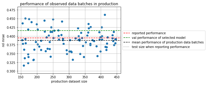
monitor production

observe that even when showing NEW data to our selected model, performance still varies.

as we have more data kept in this dataset we SIMULATE we get new data batches from production.

in SMALL DATA performance biases are DIFFICULT to overcome in practice and must be monitored!!!

how much data is small data depends on your problem.

er = []
sizes = []
for _ in range(100):
    size = len(Xts)+np.random.randint(len(Xts))-len(Xts)//2
    ed = dataset.iloc[10000:].sample(size)
    eX = ed.values[:,:-1]
    ey = ed["medianHouseValue"].values
    er.append(rel_mrae(best_estimator, eX, ey))
    sizes.append(size)

plt.scatter(sizes, er)
plt.xlabel("production dataset size")
plt.ylabel("rel mrae")
plt.title("performance of observed data batches in production")
plt.axhline(reported_performance, color="red", ls="--", label="reported performance")
plt.axhline(zscores[best], color="green", ls="--", label="val performance of selected model")
plt.axhline(np.mean(er), color="black", ls="--", label="mean performance of production data batches")
plt.axvline(len(Xts), color="black", alpha=.5, ls=":", label="test size when reporting performance")
plt.grid(); plt.legend(loc='center left', bbox_to_anchor=(1, 0.5));

suggested experiment

change test_size and number_of_houses_for_trainval when using train/val/test splits above

larger values might yield better stability of results