02.03 - NUMPY#
!wget --no-cache -O init.py -q https://raw.githubusercontent.com/rramosp/ai4eng.v1/main/content/init.py
import init; init.init(force_download=False); init.get_weblink()
import numpy as np
numpy is mostly about matrix data manipulation#
see this cheat sheet: https://s3.amazonaws.com/assets.datacamp.com/blog_assets/Numpy_Python_Cheat_Sheet.pdf
Python lists do not implement matrix semantics
a = [ 1, 2, 3]
b = [10,20,30]
a + b
[1, 2, 3, 10, 20, 30]
a = np.array([1,2,3])
b = np.array([10,20,30])
a + b
array([11, 22, 33])
Many ways of creating arrays#
# manually
a = np.array([[1,2,3],[4,5,6]])
a
array([[1, 2, 3],
       [4, 5, 6]])
# random creation
a = np.random.random(size=(3,5))
a
array([[0.55440071, 0.6683425 , 0.04754402, 0.10139782, 0.62052393],
       [0.85280182, 0.14129181, 0.02150629, 0.74116705, 0.54279996],
       [0.44723113, 0.88703075, 0.69994273, 0.08053102, 0.29767636]])
a = np.random.normal(size=(2,3,4))
a
array([[[-1.38678957,  0.17539717, -0.58164117, -0.07952217],
        [-0.18639307,  0.89132022,  0.15618823,  1.21764204],
        [-1.4800378 ,  0.80113909,  0.35547133,  0.10331395]],

       [[ 0.16612443,  0.63344446, -0.73897797, -1.76982784],
        [-1.06779833,  0.25467552,  0.57457527, -0.35351982],
        [ 0.72183531, -1.48463896, -1.40550808, -0.84931148]]])
a = np.random.randint(100, size=(4,10))
a
array([[57, 19, 49, 57, 49, 22, 41, 41, 16, 66],
       [46, 94, 86, 88, 13, 21,  8, 43,  2, 12],
       [48, 74, 12, 42, 34, 19, 59, 72, 18, 21],
       [32,  9, 25, 33, 30, 89, 24, 18, 72, 13]])
# deterministic
np.eye(3)
array([[1., 0., 0.],
       [0., 1., 0.],
       [0., 0., 1.]])
np.linspace(-3,20,10)
array([-3.        , -0.44444444,  2.11111111,  4.66666667,  7.22222222,
        9.77777778, 12.33333333, 14.88888889, 17.44444444, 20.        ])
np.arange(-3,20)
array([-3, -2, -1,  0,  1,  2,  3,  4,  5,  6,  7,  8,  9, 10, 11, 12, 13,
       14, 15, 16, 17, 18, 19])
np.arange(-3,2)
array([-3, -2, -1, 0, 1])
np.zeros((5,10))
array([[0., 0., 0., 0., 0., 0., 0., 0., 0., 0.],
       [0., 0., 0., 0., 0., 0., 0., 0., 0., 0.],
       [0., 0., 0., 0., 0., 0., 0., 0., 0., 0.],
       [0., 0., 0., 0., 0., 0., 0., 0., 0., 0.],
       [0., 0., 0., 0., 0., 0., 0., 0., 0., 0.]])
np.ones((5,10))
array([[1., 1., 1., 1., 1., 1., 1., 1., 1., 1.],
       [1., 1., 1., 1., 1., 1., 1., 1., 1., 1.],
       [1., 1., 1., 1., 1., 1., 1., 1., 1., 1.],
       [1., 1., 1., 1., 1., 1., 1., 1., 1., 1.],
       [1., 1., 1., 1., 1., 1., 1., 1., 1., 1.]])
Info on arrays#
a = np.random.randint(100, size=(3,4))
a
array([[27,  8, 66, 31],
       [95, 99, 93, 25],
       [41, 65, 25, 35]])
a.shape, len(a)
((3, 4), 3)
len(a.shape)
2
a.size
12
a.dtype
dtype('int64')
b = a.astype(np.float32)
b
array([[27.,  8., 66., 31.],
       [95., 99., 93., 25.],
       [41., 65., 25., 35.]], dtype=float32)
Operations with arrays#
element by element
a = np.array([3,5,4])
b = np.array([10,5,30])
a + b
array([13, 10, 34])
a * b
array([ 30, 25, 120])
b ** a
array([ 1000, 3125, 810000])
np.sin(a)
array([ 0.14112001, -0.95892427, -0.7568025 ])
a == b
array([False, True, False])
matrix operations
a.sum()
12
np.sum(a), np.max(a), np.min(a), np.mean(a), np.std(a), np.product(a)
(12, 5, 3, 4.0, 0.816496580927726, 60)
a.dot(b)
175
np.sum(a*b)
175
a = np.random.randint(100, size=(3,4))
a
array([[40, 53, 88, 22],
       [31, 82, 72, 87],
       [13, 91, 62, 16]])
a.T
array([[40, 31, 13],
       [53, 82, 91],
       [88, 72, 62],
       [22, 87, 16]])
a = np.array([3,5,4])
b = np.array([10,5,30])
np.allclose(a,b)
False
np.any(a==b)
True
Indexing#
a = np.random.randint(100, size=(6,10))
a
array([[ 3, 38, 63, 87, 55, 49, 96, 63, 31, 14],
       [96, 66, 85, 64, 53,  5,  4, 57, 70, 88],
       [15, 73, 67, 47, 94, 60, 34, 73, 35, 92],
       [66, 95, 47, 75, 97, 60, 24, 52, 36,  3],
       [62, 11,  1, 64, 94, 32, 68, 33, 74, 84],
       [72, 60, 11, 92, 47, 13,  4, 49, 67, 50]])
a[1]
array([96, 66, 85, 64, 53, 5, 4, 57, 70, 88])
a[:,1]
array([38, 66, 73, 95, 11, 60])
a[1,:]
array([96, 66, 85, 64, 53, 5, 4, 57, 70, 88])
a[:3]
array([[ 3, 38, 63, 87, 55, 49, 96, 63, 31, 14],
       [96, 66, 85, 64, 53,  5,  4, 57, 70, 88],
       [15, 73, 67, 47, 94, 60, 34, 73, 35, 92]])
a[:,3:8]
array([[87, 55, 49, 96, 63],
       [64, 53,  5,  4, 57],
       [47, 94, 60, 34, 73],
       [75, 97, 60, 24, 52],
       [64, 94, 32, 68, 33],
       [92, 47, 13,  4, 49]])
a[2:-1,3:-2]
array([[47, 94, 60, 34, 73],
       [75, 97, 60, 24, 52],
       [64, 94, 32, 68, 33]])
boolean indices
a = np.random.randint(100, size=(10))
a
array([67, 64, 72, 24, 45, 90, 98, 64, 73, 33])
a[[ True, True, False, False, False, False, True, False, False, False]]
array([67, 64, 98])
a<50
array([False, False, False,  True,  True, False, False, False, False,
        True])
a[a<50]
array([24, 45, 33])
a[(a<50)&(a%2==0)]
array([24])
Axis operations#
a = np.random.randint(100, size=(6,10))
a
array([[ 3,  6, 28, 26, 24, 12, 63, 14, 14, 60],
       [97, 45, 63, 40, 83, 83, 21, 49, 20, 47],
       [53, 35, 72, 83, 62, 92, 20, 65,  1, 71],
       [79, 69, 55, 91, 34, 88, 28,  1, 50, 26],
       [82, 62, 37, 76, 94, 13, 21, 16, 42, 17],
       [99, 72, 52, 85,  3, 57, 66, 86, 97, 91]])
np.max(a, axis=0)
array([99, 72, 72, 91, 94, 92, 66, 86, 97, 91])
np.max(a, axis=1)
array([63, 97, 92, 91, 94, 99])
np.mean(a, axis=1)
array([25. , 54.8, 55.4, 52.1, 46. , 70.8])
np.argmax(a, axis=1)
array([6, 0, 5, 3, 4, 0])
reshaping is very useful
a.shape
(6, 10)
a.reshape(5,12)
array([[ 3,  6, 28, 26, 24, 12, 63, 14, 14, 60, 97, 45],
       [63, 40, 83, 83, 21, 49, 20, 47, 53, 35, 72, 83],
       [62, 92, 20, 65,  1, 71, 79, 69, 55, 91, 34, 88],
       [28,  1, 50, 26, 82, 62, 37, 76, 94, 13, 21, 16],
       [42, 17, 99, 72, 52, 85,  3, 57, 66, 86, 97, 91]])
a.reshape(5,-1)
array([[ 3,  6, 28, 26, 24, 12, 63, 14, 14, 60, 97, 45],
       [63, 40, 83, 83, 21, 49, 20, 47, 53, 35, 72, 83],
       [62, 92, 20, 65,  1, 71, 79, 69, 55, 91, 34, 88],
       [28,  1, 50, 26, 82, 62, 37, 76, 94, 13, 21, 16],
       [42, 17, 99, 72, 52, 85,  3, 57, 66, 86, 97, 91]])
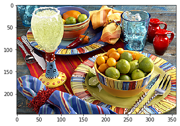
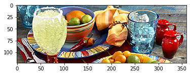
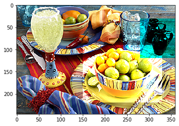
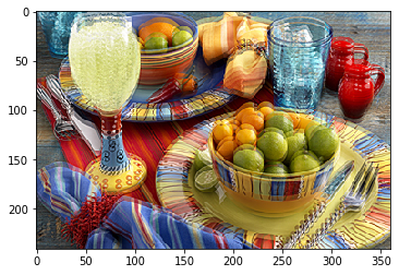
Many things can be represented by matrices. For instance, images#
from skimage import io
import matplotlib.pyplot as plt
%matplotlib inline
img = io.imread("local/imgs/sample_img.jpg")
type(img)
numpy.ndarray
img.shape
(246, 360, 3)
np.min(img), np.max(img)
(0, 255)
convert it to standard [0,1] range
img = img/255
np.min(img), np.max(img)
(0.0, 1.0)
plt.imshow(img)
<matplotlib.image.AxesImage at 0x7fba1095fa50>
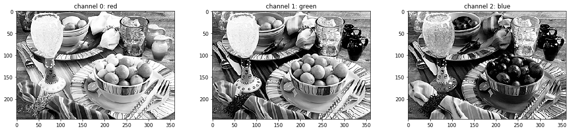
observe the channel composition of the image: lighter \(\rightarrow\) greater color presence
cnames = ["red", "green", "blue"]
plt.figure(figsize=(20,4))
for i in range(3):
    plt.subplot(1,3,i+1)
    plt.imshow(img[:,:,i], plt.cm.Greys_r)
    plt.title("channel %i: %s"%(i, cnames[i]))
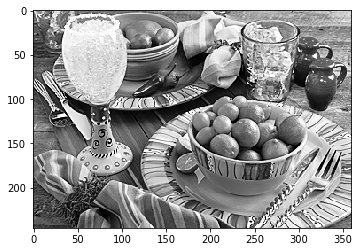
grayscale version
plt.imshow(np.mean(img, axis=2), plt.cm.Greys_r)
<matplotlib.image.AxesImage at 0x7fba0dd86810>
plt.imshow(img[:img.shape[0]//2,:,:])
<matplotlib.image.AxesImage at 0x7fba0dd74450>
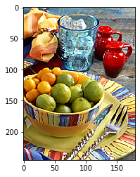
plt.imshow(img[:,img.shape[1]//2:,:])
<matplotlib.image.AxesImage at 0x7fba0dcdf950>
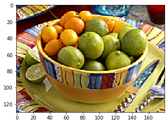
plt.imshow(img[90:220, 150:330,:])
<matplotlib.image.AxesImage at 0x7fba0de144d0>
copy an array
img2 = img.copy()
id(img), id(img2)
(140437109691936, 140437104473072)
increase luminosity
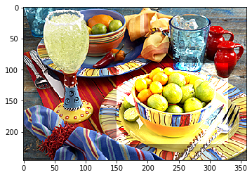
img2[90:220, 150:330,:] *= 2
plt.imshow(img2)
Clipping input data to the valid range for imshow with RGB data ([0..1] for floats or [0..255] for integers).
<matplotlib.image.AxesImage at 0x7fba0f731390>
remove channel
img2[30:120, 280:, 0] = 0
plt.imshow(img2)
Clipping input data to the valid range for imshow with RGB data ([0..1] for floats or [0..255] for integers).
<matplotlib.image.AxesImage at 0x7fba0deb2490>
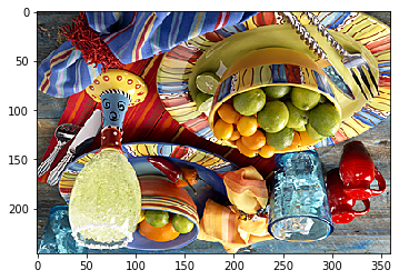
plt.imshow(img[::-1,:,:])
<matplotlib.image.AxesImage at 0x7fba0dc5d3d0>
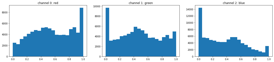
understand luminosity on each channel
img.flatten().shape
(265680,)
img[:,:,0].flatten().shape
(88560,)
cnames = ["red", "green", "blue"]
plt.figure(figsize=(20,4))
for i in range(3):
    plt.subplot(1,3,i+1)
    plt.hist(img[:,:,i].flatten(), bins=20);
    plt.title("channel %i: %s"%(i, cnames[i]))
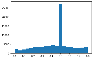
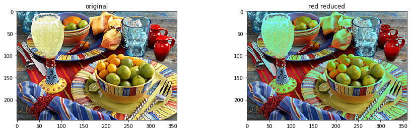
reduce luminosity on red channel
img3 = img.copy()
img3[:,:,0][img3[:,:,0]>0.8] = 0.5
plt.hist(img3[:,:,0].flatten(), bins=20);
plt.figure(figsize=(15,4))
plt.subplot(121); plt.imshow(img); plt.title("original")
plt.subplot(122); plt.imshow(img3); plt.title("red reduced")
Text(0.5, 1.0, 'red reduced')
shift and overlap
img4 = (img[5:,:,:] + img[:-5:,:,:])/2
plt.imshow(img4)
<matplotlib.image.AxesImage at 0x7fba0d89af90>
img3.shape, img.shape
((246, 360, 3), (246, 360, 3))
Vectorization#
exploit numpy vectorized operations, avoid for loops as much as possible
a = np.random.randint(100, size=(6,10))
a
array([[40,  5,  3,  4, 65, 21, 64, 31, 83,  2],
       [74, 65, 28, 43, 29, 42, 48, 84,  2, 79],
       [62, 36,  3, 92, 16, 48, 88, 40, 58,  7],
       [92, 70, 67,  1, 64, 77, 35, 81, 66, 15],
       [20,  8, 20, 66, 66,  9, 98, 35, 45, 79],
       [ 8, 79, 64, 72, 41, 63, 34, 58, 35, 53]])
np.mean(a, axis=1)
array([31.8, 49.4, 45. , 56.8, 44.6, 50.7])
np.array([np.mean(a[i,:]) for i in range(a.shape[0])])
array([31.8, 49.4, 45. , 56.8, 44.6, 50.7])
%timeit np.mean(a, axis=1)
9.19 µs ± 1.22 µs per loop (mean ± std. dev. of 7 runs, 100000 loops each)
%timeit np.array([np.mean(a[i,:]) for i in range(a.shape[0])])
44 µs ± 7.28 µs per loop (mean ± std. dev. of 7 runs, 10000 loops each)
always think if oyu can vectorize. For instance, for two (large) matrices
a = np.random.randint(100, size=(1000,100))
b = np.random.randint(200, size=(1000,100))
the number of elements which are the equal
np.mean(a==b)
0.00482
The mean of the elements of a that are greater to its corresponding position in b
np.mean(a[a>b])
66.20718043452071
The mean of the elements of b that are greater to its corresponding position in a
np.mean(b[b>a])
121.86164010882239
with smaller matrices
a = np.random.randint(100, size=(10))
b = np.random.randint(200, size=(10))
print (a)
print (b)
[26 46 68 37  9 86 16  4 63  8]
[  1  59  96  35  91  29 196 178 195  61]
the element in b corresponding to the position of the greatest element in a
b[np.argmax(a)]
29
Broadcasting#
usually numpy needs matrix dimensions to match when doing operations among them
a = np.random.randint(100, size=(3,5))
b = np.random.randint(10, size=(3,4))
print (a)
print (b)
a + b
[[70 62 73 18  3]
 [99 19 41 31 24]
 [81 73 72 49  9]]
[[7 6 5 9]
 [1 2 6 7]
 [9 3 5 2]]
---------------------------------------------------------------------------
ValueError                                Traceback (most recent call last)
<ipython-input-89-860cc8167430> in <module>
      3 print (a)
      4 print (b)
----> 5 a + b

ValueError: operands could not be broadcast together with shapes (3,5) (3,4)
but numpy tries to expand the operations if some dimensions match
a
array([[70, 62, 73, 18,  3],
       [99, 19, 41, 31, 24],
       [81, 73, 72, 49,  9]])
a*10
array([[700, 620, 730, 180,  30],
       [990, 190, 410, 310, 240],
       [810, 730, 720, 490,  90]])
observe the reshape in the following operation
a + b[:,1].reshape(-1,1)
array([[ 76,  68,  79,  24,   9],
       [101,  21,  43,  33,  26],
       [ 84,  76,  75,  52,  12]])
b[:,1].reshape(-1,1)
array([[6],
       [2],
       [3]])
b[:,1]
array([6, 2, 3])
a + b[:,1]
---------------------------------------------------------------------------
ValueError                                Traceback (most recent call last)
<ipython-input-95-d148e74cc6fe> in <module>
----> 1 a + b[:,1]

ValueError: operands could not be broadcast together with shapes (3,5) (3,)
observe row wise
a + b.flatten()[:a.shape[1]]
array([[ 77,  68,  78,  27,   4],
       [106,  25,  46,  40,  25],
       [ 88,  79,  77,  58,  10]])
print (a)
print (b)
[[70 62 73 18  3]
 [99 19 41 31 24]
 [81 73 72 49  9]]
[[7 6 5 9]
 [1 2 6 7]
 [9 3 5 2]]
b.flatten()
array([7, 6, 5, 9, 1, 2, 6, 7, 9, 3, 5, 2])
b.flatten()[:a.shape[1]]
array([7, 6, 5, 9, 1])
Functions args by reference#
except scalar, function arguments are always passed by reference
if you modify it within a function it will change
the name within a function can be different, but will point to the same object
observe the difference if the following expressions (showing with numpy arrays, not general in python)
a = np.round(np.random.random(size=5),3)
print (a)
id(a)
[0.714 0.774 0.671 0.681 0.654]
140437066859584
a = a + 1
print (a)
id(a)
[1.714 1.774 1.671 1.681 1.654]
140437066861584
this operation is semantically the same, but it produces a different memory footprint (faster, no copy, modifies in place)
a += 1
print (a)
id(a)
[2.714 2.774 2.671 2.681 2.654]
140437066861584
now in functions
a = np.round(np.random.random(size=5),3)
print (a)
id(a)
[0.801 0.023 0.035 0.148 0.896]
140437067580640
def getmax(x):
    print ("mem address in function", id(x))
    return np.max(x)
getmax(a)
mem address in function 140437067580640
0.896
def getmax_after_sinplus1(x):
    print ("mem address in function before op", id(x))
    x = np.sin(x+1)
    print ("mem address in function after op", id(x))
    return np.max(x)
getmax_after_sinplus1(a)
mem address in function before op 140437067580640
mem address in function after op 140437067620224
0.9736199418975943
print (a)
[0.801 0.023 0.035 0.148 0.896]
however, the following implementation changes a outside the function
def getmax_after_sinplus1(x):
    print ("mem address in function before op", id(x))
    x += 1
    print ("mem address in function after +1", id(x))
    x = np.sin(x)
    print ("mem address in function after sin", id(x))
    return np.max(x)
getmax_after_sinplus1(a)
mem address in function before op 140437067580640
mem address in function after +1 140437067580640
mem address in function after sin 140437067015232
0.9736199418975943
print (a)
[1.801 1.023 1.035 1.148 1.896]
Expressions like +1 are faster and use less memory but may have side effects. We will see this in pandas
Matplotlib#
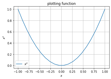
plotting naturally exploits vectorization
see https://matplotlib.org/gallery.html for exameples and guides.
x = np.linspace(-1,1,20)
x
array([-1.        , -0.89473684, -0.78947368, -0.68421053, -0.57894737,
       -0.47368421, -0.36842105, -0.26315789, -0.15789474, -0.05263158,
        0.05263158,  0.15789474,  0.26315789,  0.36842105,  0.47368421,
        0.57894737,  0.68421053,  0.78947368,  0.89473684,  1.        ])
x**2
array([1.        , 0.80055402, 0.6232687 , 0.46814404, 0.33518006,
       0.22437673, 0.13573407, 0.06925208, 0.02493075, 0.00277008,
       0.00277008, 0.02493075, 0.06925208, 0.13573407, 0.22437673,
       0.33518006, 0.46814404, 0.6232687 , 0.80055402, 1.        ])
plt.plot(x, x**2, label="$x^2$")
# cosmetics
plt.grid();
plt.title("plotting function")
plt.xlabel("$x$")
plt.ylabel("$x^2$")
plt.legend();
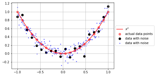
all plotting happens in the same figure until we create a new one
plt.plot(x, x**2, color="red", label="$x^2$")

x2_with_noise = x**2 + np.random.normal(size=x.shape)*.1

xdense = np.linspace(np.min(x), np.max(x), 200)
xdense2_with_noise = xdense**2 + np.random.normal(size=xdense.shape)*.1


plt.scatter(x, x**2, s=50, color="red", alpha=.5, label="actual data points")
plt.scatter(x, x2_with_noise, s=50, color="black", label="data with noise")
plt.scatter(xdense, xdense2_with_noise, s=5, color="blue", alpha=.5, label="data with noise")
plt.grid();

plt.legend(loc='center left', bbox_to_anchor=(1, 0.5))
<matplotlib.legend.Legend at 0x7fba1043ac10>
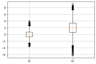
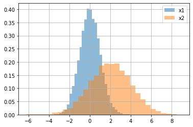
some statistical plots
x1 = np.random.normal(loc=0, scale=1, size=10000)
x2 = np.random.normal(loc=2, scale=2, size=10000)
plt.hist(x1, bins=30, alpha=.5, density=True, label="x1");
plt.hist(x2, bins=30, alpha=.5, density=True, label="x2");
plt.grid(); plt.legend();
plt.boxplot([x1, x2]);
plt.grid();
plt.xticks(range(1,3), ["x1", "x2"]);