04.04 - COMPARING SAMPLES

!wget --no-cache -O init.py -q https://raw.githubusercontent.com/rramosp/ai4eng.v1/main/content/init.py
import init; init.init(force_download=False); init.get_weblink()

endpoint https://m5knaekxo6.execute-api.us-west-2.amazonaws.com/dev-v0001/rlxmooc

See my courses and progress

from scipy import stats
import numpy as np
import matplotlib.pyplot as plt
from progressbar import progressbar as pbar
%matplotlib inline

Comparing populations. A two-sided test

We have some exam scores for two groups of 10 students each

STEP 1: Define the model you want to challenge (the NULL Hypothesis \(H_0\))

We define the \(H_0\) as a model where there is no statistical difference between the two groups of students.

STEP 2: Define your REAL WORLD sample and your test statistic

• SAMPLE: we sample two groups of 10 students exam scores each. We KNOW there is a difference (mean_diff) because we create the use case in such way. We want to see if the test detects it.

  • Can it detect it with larger/smaller group sizes?

  • Can it detect it with larger/smaller mean differences?

real_world_sample_size = 10
mu, sigma = 100, 10

def generate_AB(mu=mu, sigma=sigma, real_world_sample_size=real_world_sample_size, mean_diff=5):
    A = np.random.normal(loc=mu, scale=sigma, size=real_world_sample_size)
    B = np.random.normal(loc=mu+mean_diff, scale=sigma, size=real_world_sample_size)
    return A, B

A,B = generate_AB()
print ("group A  [", " ".join(["%6.2f"%i for i in A]), "]  mean %6.2f"%np.mean(A))
print ("group B  [", " ".join(["%6.2f"%i for i in B]), "]  mean %6.2f"%np.mean(B))

group A  [  96.08 101.76  89.45  88.81 106.66 105.94  95.99 108.45  94.67 114.32 ]  mean 100.21
group B  [ 129.23 127.05 115.34 105.17 117.75 121.96 103.69 120.42 118.77  89.56 ]  mean 114.89

if we look at these two sets of scores, how sure can we be that their respective populations are different (different \(\mu\))?

Define a test statistic to measure the mean difference of the samples

\[\text{ttest}(A,B) = \frac{\bar{A}-\bar{B}}{\sqrt{\frac{S_A^2}{N_A}+\frac{S_B^2}{N_B}}}\]

where:

• \(\bar{A}\), \(\bar{B}\) is the mean of the two real world samples

• \(S_A\), \(S_B\) is the standard deviation of the two real world samples

• \(N_A\), \(N_B\) is the size (number of elementso) of the two real world samples

The denominator factor is included so that we can compare the means with different standard deviations.

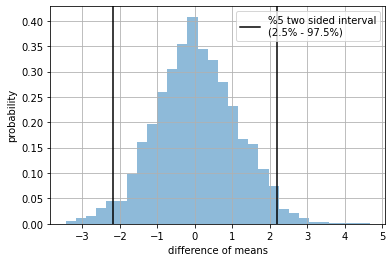
STEP 3: We simulate \(H_0\), and understand its distribution of \(\text{ttest}\)

individual student scores NEED NOT come from a normal disitribution. Regardless their origin, the distribution of the test statistic will be normal.

ttest = lambda a,b: (np.mean(a)-np.mean(b))/np.sqrt(np.std(a)**2/len(a)+np.std(b)**2/len(b))

n = 3000

a = np.r_[[stats.norm(loc=mu, scale=sigma).rvs(real_world_sample_size) for _ in pbar(range(n))]]
b = np.r_[[stats.norm(loc=mu, scale=sigma).rvs(real_world_sample_size) for _ in pbar(range(n))]]

t = np.r_[[ttest(i,j) for i,j in zip(a,b)]]

100% (3000 of 3000) |####################| Elapsed Time: 0:00:01 Time:  0:00:01
100% (3000 of 3000) |####################| Elapsed Time: 0:00:01 Time:  0:00:01

# A,B = generate_AB()

plt.hist( t, density=True, alpha=.5, bins=30);
plt.axvline(np.percentile(t,2.5), color="black", label="%5 two sided interval\n(2.5% - 97.5%) ")
plt.axvline(np.percentile(t,97.5), color="black")
plt.grid(); plt.legend(); 
plt.xlabel("difference of means"); plt.ylabel("probability")
plt.show()

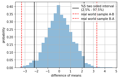
STEP 5: How rare is our real world sample w.r.t. \(H_0\)?

we measure how much probability mass is left outside the red dashed lines (our real world sample)

• small \(p_{value}\) means our real world sample is rare

• large \(p_{value}\) means our real world sample is quite common (expected)

For a confidence interval \(\alpha=0.05\), if \(p_{value}<\alpha\) we reject \(H_0\) and consider \(A\) and \(B\) actually come from different populations.

observe we display \(\text{ttest}(A,B)\) and \(\text{ttest}(B,A)\) (red dashed lines) since we want to check if they are different in any direction

print ("group A  [", " ".join(["%6.2f"%i for i in A]), "]  mean %6.2f"%np.mean(A))
print ("group B  [", " ".join(["%6.2f"%i for i in B]), "]  mean %6.2f"%np.mean(B))


plt.hist( t, density=True, alpha=.5, bins=30);
plt.axvline(np.percentile(t,2.5), color="black", label="%5 two sided interval\n(2.5% - 97.5%) ")
plt.axvline(np.percentile(t,97.5), color="black")
plt.axvline(ttest(A,B), color="red", ls="--", label="real world sample A-B")
plt.axvline(ttest(B,A), color="red", ls="--", label="real world sample B-A")
plt.grid(); plt.legend(); 
plt.xlabel("difference of means"); plt.ylabel("probability")
plt.show()

group A  [  96.08 101.76  89.45  88.81 106.66 105.94  95.99 108.45  94.67 114.32 ]  mean 100.21
group B  [ 129.23 127.05 115.34 105.17 117.75 121.96 103.69 120.42 118.77  89.56 ]  mean 114.89

#A,B = generate_AB()

k = np.mean( ttest(A,B)<t)
k = (k if k<0.5 else 1-k)*2
print ("empirical (simulated) p-value %.4f"%k)

empirical (simulated) p-value 0.0013

which corresponds to the value obtained with the analytical formula

As implemented in scipy.stats.ttest_ind. With larger simulations, the result gets closer to the analytical formula.

stats.ttest_ind(A, B).pvalue

0.005726493310989277

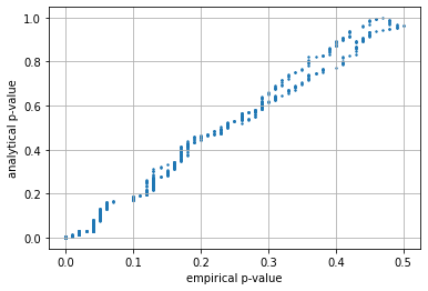
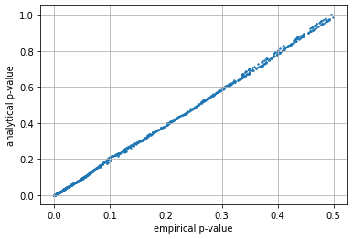
Understanding accuracy of large and small simulations

observe the relation between the empirical (simulated) and analytical \(p_{value}\) is much tighter (more accurate) when the simulation is larger.

    
def test_simulations(n, mu=mu, sigma=sigma, real_world_sample_size=real_world_sample_size):
    a = np.r_[[stats.norm(loc=mu, scale=sigma).rvs(real_world_sample_size) for _ in pbar(range(n))]]
    b = np.r_[[stats.norm(loc=mu, scale=sigma).rvs(real_world_sample_size) for _ in pbar(range(n))]]

    t = np.r_[[ttest(A, B) for A,B in zip(a,b)]]
    r = []
    for _  in range(1000):
        A,B = generate_AB(mu=mu, sigma=sigma, real_world_sample_size=real_world_sample_size)
        ts = ttest(A,B)
        
        k = np.mean( ts<t)
        k = (k if k<0.5 else 1-k)*2
        r.append([k, stats.ttest_ind(A, B).pvalue])
    r = np.r_[r]
    
    plt.scatter(r[:,0], r[:,1], s=2)
    plt.grid(); plt.xlabel("empirical p-value"); plt.ylabel("analytical p-value")
    
    em, an = r[:,0], r[:,1]
    
    print ("p_value mean error simulated/analytic %.3f"%np.mean(np.abs(em-an)))
    print ("p_value mean error when p_value<0.05  %.3f"%np.mean(np.abs(em[an<0.05]-an[an<0.05])))

test_simulations(n=100, mu=mu, sigma=sigma)

100% (100 of 100) |######################| Elapsed Time: 0:00:00 Time:  0:00:00
100% (100 of 100) |######################| Elapsed Time: 0:00:00 Time:  0:00:00

p_value mean error simulated/analytic 0.165
p_value mean error when p_value<0.05  0.004

test_simulations(n=1000, mu=mu, sigma=sigma)

100% (1000 of 1000) |####################| Elapsed Time: 0:00:00 Time:  0:00:00
100% (1000 of 1000) |####################| Elapsed Time: 0:00:00 Time:  0:00:00

p_value mean error simulated/analytic 0.172
p_value mean error when p_value<0.05  0.016

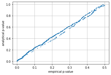
test_simulations(n=6000, mu=mu, sigma=sigma)

100% (6000 of 6000) |####################| Elapsed Time: 0:00:02 Time:  0:00:02
100% (6000 of 6000) |####################| Elapsed Time: 0:00:02 Time:  0:00:02

p_value mean error simulated/analytic 0.168
p_value mean error when p_value<0.05  0.009

For more info:

• Sampling distribution of the sample mean Khan Academy

• Central limit theorem Wikipedia

Refs

• scipy.stats.ttest_ind

• Wikipedia T-test