07.03 - NEURAL NETWORKS#
!wget --no-cache -O init.py -q https://raw.githubusercontent.com/rramosp/ai4eng.v1/main/content/init.py
import init; init.init(force_download=False); init.get_weblink()
import numpy as np
import matplotlib.pyplot as plt
from local.lib import mlutils
from IPython.display import Image
%matplotlib inline
Reinterpreting logistic regression#
observe how we can represent the same logistic regression expression we saw before.
## KEEPOUTPUT
Image("local/imgs/logreg.png", width=600)
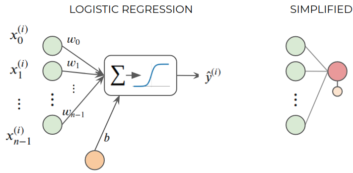
This also goes by the weird name of The Perceptron
Recall that matrix and vector multiplication and numpybroadcasting are very convenient to make this operation for a single element or for the full dataset.
with
See and understand this with the following random dataset (\(\mathbf{X}\)) and parameters (\(\theta\)).
\(m\) is the number of data items we have (rows), and \(n\) is the number of attributes per data point (columns).
This can be seen as a EXTREME SIMPLIFICATION of a biological neuron.
## KEEPOUTPUT
m,n = 1000,5
X = np.random.normal(size=(m,n))
t = np.random.normal(size=n)
b = np.random.normal()

sigmoid = lambda z: 1/(1+np.exp(-z))

print ("X\n",X)
print ("\n\nt\n", t)
print ("\n\nb\n", b)
X.shape, t.shape
X
 [[-0.3587495   0.32494874  0.85232788  1.35268481 -0.43819386]
 [-0.14368593 -0.20965451  1.41444411 -1.16854331  1.62431814]
 [-1.8191772  -1.08488133 -1.23953431 -1.68329863  1.25165422]
 ...
 [-0.92844069 -1.13526592  1.09861043  0.7697974   0.0805227 ]
 [-0.60019426 -0.53171841  0.40924603  0.23610253  0.51590451]
 [-0.90455498  0.59690779  0.38095951  1.41948005  0.1054254 ]]


t
 [-2.82751082  0.27325313  1.18576235  0.16695059  0.73230592]


b
 -0.41753312455308067
((1000, 5), (5,))
logistic regression prediction in one line of code for the full dataset
## KEEPOUTPUT
y_hat = sigmoid(X.dot(t)+b)

print (y_hat[:10])
y_hat.shape
[0.83218968 0.93105794 0.97328719 0.73485156 0.76756293 0.95789916
 0.03590429 0.68380291 0.12493222 0.24181324]
(1000,)
Neural networks \(\rightarrow\) Assembling logistic regression units#
we can have several perceptrons together from the same input
## KEEPOUTPUT
Image("local/imgs/mlp.png", width=600)
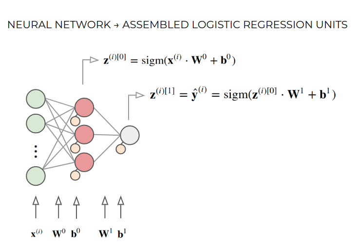
what are the sizes of the symbols above? HINT: Matrix multiplication has to match up.
\(\mathbf{x}^{(i)} \;\;\;\in \mathbb{R}^n\)
\(\mathbf{W}^0 \;\;\;\in \mathbb{R}^{n\times 3}\rightarrow\;\;\)each column contains the weights of one logistic regression unit.
\(\mathbf{b}^0 \;\;\;\;\in \mathbb{R}^3\;\;\;\rightarrow\;\;\)one per logistic regression unit.
\(\mathbf{z}^{(i)[0]} \in \mathbb{R}^3\;\;\;\rightarrow\;\;\)one output per logistic regression unit.
\(\mathbf{W}^1 \;\;\in \mathbb{R}^{3}\;\;\;\rightarrow\;\;\)this is a regular logistic regression unit, but its input comes from the previous layer.
\(\mathbf{b}^1 \; \;\;\in \mathbb{R}\;\;\;\;\;\rightarrow\;\;\)like a regular logistic regression unit.
\(\hat{y}^{(i)}\; \;\in \mathbb{R}\;\;\;\;\;\rightarrow\;\;\)the network output
we can have different activations functions
\(\mathbf{z}^{(i)[0]} = \text{tanh}(\mathbf{x}^{(i)}\cdot \mathbf{W}^0+\mathbf{b}^0)\)
\(\mathbf{z}^{(i)[1]} = \hat{\mathbf{y}}^{(i)} = \text{sigm}(\mathbf{z}^{(i)[0]}\cdot \mathbf{W}^1+\mathbf{b}^1)\)
sigmoid = lambda z: 1/(1+np.exp(-z))
relu    = lambda z: z*(z>0)
## KEEPOUTPUT
xr = np.linspace(-10,10,100)
plt.figure(figsize=(15,3))
plt.subplot(131)
plt.axhline(0, color="black")
plt.axvline(0, color="black")
plt.plot(xr, sigmoid(xr) ,lw=2)
plt.grid();
plt.title("sigmoid function")

plt.subplot(132)
plt.axhline(0, color="black")
plt.axvline(0, color="black")
plt.plot(xr, np.tanh(xr) ,lw=2)
plt.grid();
plt.title("tanh function")

plt.subplot(133)
plt.axhline(0, color="black")
plt.axvline(0, color="black")
plt.plot(xr, relu(xr) ,lw=2)
plt.grid();
plt.title("relu function")
Text(0.5, 1.0, 'relu function')
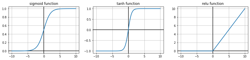
in general
\(\text{sigm}\) is good for output units (can be interpreted as probability)
\(\text{tanh}\) is good for hidden layers in small networks (neg and pos contributions)
\(\text{relu}\) is good for hidden layers is large (deep learning) networks (easier to train)
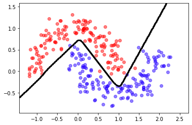
Observe the capacity of neural networks to create classification frontiers.
The following set of weights were obtained AFTER training a neural network with the sklearn moons dataset:
input data has two columns
the hidden layer has four neurons (logistic units)
Try to understant the shapes as we are computing ALL predictions for a dataset SIMULTANEOUSLY, using numpy vectorized operations.
## KEEPOUTPUT
b0,b1,W0,W1 = (np.array([-12.89987776,  10.35173209,  11.65978321,  -7.55016811]),
              -17.36405931876728,
 np.array([[19.04548787, -8.65065699, 14.28282749, -9.44291219],
        [15.44773976,  5.09753522, -3.12074945, 10.5002505 ]]),
 np.array([-42.17763359,-34.87459471, 7.21432064,-36.52606503]))

print ("W0:\n",W0)
print ("\nb0:\n",b0)
print ("\nW1:\n",W1)
print ("\nb1:\n",b1)

W0.shape, b0.shape, W1.shape, type(b1)
W0:
 [[19.04548787 -8.65065699 14.28282749 -9.44291219]
 [15.44773976  5.09753522 -3.12074945 10.5002505 ]]

b0:
 [-12.89987776  10.35173209  11.65978321  -7.55016811]

W1:
 [-42.17763359 -34.87459471   7.21432064 -36.52606503]

b1:
 -17.36405931876728
((2, 4), (4,), (4,), float)
## KEEPOUTPUT
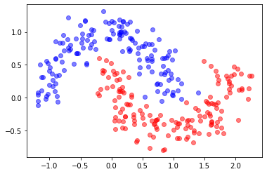
from sklearn.datasets import make_moons
X,y = make_moons(300, noise=.15)
plt.scatter(X[:,0][y==0], X[:,1][y==0], color="blue", label="class 0", alpha=.5)
plt.scatter(X[:,0][y==1], X[:,1][y==1], color="red", label="class 1", alpha=.5)
<matplotlib.collections.PathCollection at 0x7f2d86333460>
This is the NEURAL NETWORK prediction function. Observe the output is a sigmoid function and we convert it into a [0,1] classification prediction by simply threholding it at 0.5. See the sigmoid function graph above to understand why.
predict = lambda X: (sigmoid(np.tanh(X.dot(W0)+b0).dot(W1)+b1)>.5).astype(int)
from local.lib import mlutils
## KEEPOUTPUT
mlutils.plot_2Ddata_with_boundary(predict, X, y)
(0.449775, 0.550225)