05.02 - MODEL EVALUATION¶

!wget --no-cache -O init.py -q https://raw.githubusercontent.com/rramosp/ai4eng.v1/main/content/init.py
import init; init.init(force_download=False); init.get_weblink()

replicating local resources
endpoint https://m3g87w9l3k.execute-api.us-west-2.amazonaws.com/dev/rlxmooc

See my courses and progress

import numpy as np
import matplotlib.pyplot as plt
import pandas as pd
import local.lib.timeseries as ts
from local.lib import calhousing as ch
%matplotlib inline

Loading BokehJS ...

The `cal_housing` repository publicly available¶

!head local/data/cal_housing_small.data
!wc local/data/cal_housing_small.data

longitude,latitude,housingMedianAge,totalRooms,totalBedrooms,medianHouseValue
-120.58,35.0,37.0,523.0,119.0,106300.0
-118.17,33.98,31.0,1236.0,329.0,155400.0
-122.22,37.81,52.0,1971.0,335.0,273700.0
-117.91,33.66,21.0,1708.0,505.0,193800.0
-121.92,37.24,27.0,1265.0,216.0,281200.0
-117.01,32.71,20.0,3506.0,692.0,129100.0
-116.39,34.15,15.0,5583.0,1149.0,73300.0
-120.67,35.5,15.0,2752.0,546.0,175000.0
-118.18,34.04,36.0,1807.0,630.0,129000.0
  501   501 20363 local/data/cal_housing_small.data

d = pd.read_csv("local/data/cal_housing_small.data")
print (d.shape)
d.head()

(500, 6)

	longitude	latitude	housingMedianAge	totalRooms	totalBedrooms	medianHouseValue
0	-120.58	35.00	37.0	523.0	119.0	106300.0
1	-118.17	33.98	31.0	1236.0	329.0	155400.0
2	-122.22	37.81	52.0	1971.0	335.0	273700.0
3	-117.91	33.66	21.0	1708.0	505.0	193800.0
4	-121.92	37.24	27.0	1265.0	216.0	281200.0

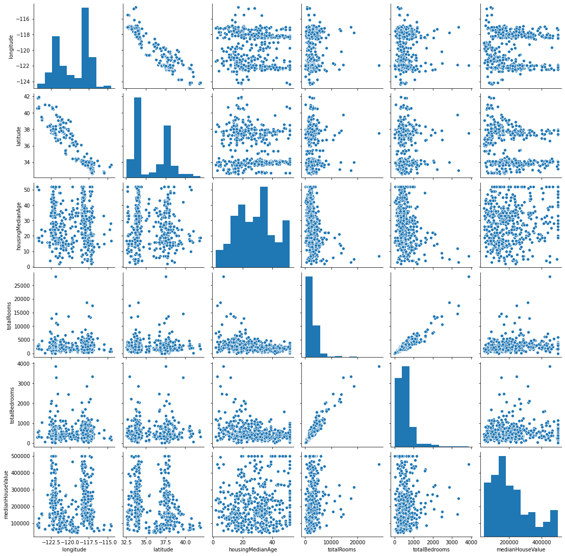
Understand data¶

import seaborn as sns
g = sns.pairplot(d)

../_images/NOTES 05.02 - MODEL EVALUATION_7_0.png

Show house locations on map¶

observa como el valor de las casas es más caro en zonas urbanas

from bokeh.plotting import *
from bokeh.models import *
import bokeh
from matplotlib import cm
from sklearn.preprocessing import MinMaxScaler

def latlng_to_meters(lat, lng):
    origin_shift = 2 * np.pi * 6378137 / 2.0
    mx = lng * origin_shift / 180.0
    my = np.log(np.tan((90 + lat) * np.pi / 360.0)) / (np.pi / 180.0)
    my = my * origin_shift / 180.0
    return mx, my


def xplot_map(lat, lon, color=None, size=10):
    cmap = cm.rainbow
    wlat, wlong = latlng_to_meters(lat, lon)
    if color is not None:
        colors = MinMaxScaler(feature_range=(0,255)).fit_transform(color)
        colors = ["#%02x%02x%02x"%tuple([int(j*255) for j in cmap(int(i))[:3]]) for i in colors]

    openmap_url = 'http://c.tile.openstreetmap.org/{Z}/{X}/{Y}.png'
    otile_url = 'http://otile1.mqcdn.com/tiles/1.0.0/sat/{Z}/{X}/{Y}.jpg'

    TILES = WMTSTileSource(url=openmap_url)
    tools="pan,wheel_zoom,reset"
    p = figure(tools=tools, min_width=700,min_height=600)

    p.add_tile(TILES)

    p.axis.visible = False

    cb = figure(min_width=40, max_width=40, min_height=600,  tools=tools)
    yc = np.linspace(np.min(color),np.max(color),20)
    c = np.linspace(0,255,20).astype(int)
    dy = yc[1]-yc[0]
    cb.rect(x=0.5, y=yc, color=["#%02x%02x%02x"%tuple([int(j*255) for j in cmap(int(i))[:3]]) for i in c], width=1, height = dy)
    cb.xaxis.visible = False
    p.circle(np.array(wlat), np.array(wlong), color=colors, size=size)
    pb = gridplot([[p, cb]])
    show(pb)

ds = d.sample(500)
xplot_map(ds["latitude"].values, 
         ds["longitude"].values, ds["medianHouseValue"].values.reshape(-1,1)/1e5) 

Separate variable to predict¶

X = d.values[:,:-1]
y = d["medianHouseValue"].values
print (X.shape, y.shape)

(500, 5) (500,)

from sklearn.linear_model import LinearRegression
from sklearn.svm import SVR
from sklearn.ensemble import RandomForestRegressor
from sklearn.model_selection import train_test_split
from sklearn.metrics import median_absolute_error, r2_score, mean_squared_error

Xtr, Xts, ytr, yts = train_test_split(X,y, test_size=0.3)
print (Xtr.shape, ytr.shape, Xts.shape, yts.shape)

(350, 5) (350,) (150, 5) (150,)

A linear regression¶

check sklearn LinearRegression doc to understand the score function.

lr = LinearRegression()
lr.fit(Xtr, ytr)
lr.score(Xtr, ytr), lr.score(Xts, yts)

(0.32232366147227454, 0.307618752063642)

r2_score(yts, lr.predict(Xts))

0.307618752063642

median_absolute_error(yts, lr.predict(Xts))

55453.23499294184

mean_squared_error(yts, lr.predict(Xts))

10000399171.317457

however we will create our score

mean releative absolute error

def rel_mrae(estimator, X, y):
    preds = estimator.predict(X)
    return np.mean(np.abs(preds-y)/y)

rel_mrae(lr, Xtr, ytr), rel_mrae(lr, Xts, yts)

(0.482339200932234, 0.3994545505967154)

let’s understand prediction errors

preds = lr.predict(Xts)
errors = np.abs(preds-yts)/yts

plt.figure(figsize=(20,3))
cols = ["longitude","latitude","housingMedianAge", "totalRooms","totalBedrooms"]
for i,col in enumerate(cols):
    plt.subplot(1,len(cols),i+1)
    plt.scatter(errors, Xts[:,i])
    plt.ylabel(col)
    plt.xlabel("relative error")
    plt.grid();

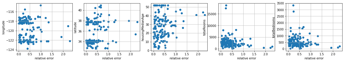
../_images/NOTES 05.02 - MODEL EVALUATION_26_0.png

we observe there is no significant correlation between the error and any. It does seem that when the houseMedianAge is smaller, the error is also smaller, and when the totalBedrooms is higher the error is also smaller. However this seems to involve only a fraction of the houses. The correlation coefficients seems to capture this.

corrcoefs = pd.DataFrame([np.corrcoef(Xts[:,i], errors)[0,1] for i in range(len(cols))], index=cols, columns=["corrcoef"])
corrcoefs

	corrcoef
longitude	-0.109087
latitude	0.172464
housingMedianAge	0.143974
totalRooms	-0.140183
totalBedrooms	-0.106749

How sure can we be of our model performance¶

resample, train and measure

bootstrap: resample and put back
cross validation: resample and partition

from progressbar import progressbar as pbar

def bootstrap_score(estimator, X, y, test_size):
  trscores, tsscores = [], []
  for _ in range(10):
    Xtr, Xts, ytr, yts = train_test_split(X,y, test_size=test_size)
    estimator.fit(Xtr, ytr)
    trscores.append(rel_mrae(estimator, Xtr, ytr))
    tsscores.append(rel_mrae(estimator, Xts, yts))

  return (np.mean(trscores), np.std(trscores)), (np.mean(tsscores), np.std(tsscores))

estimator = LinearRegression()
(trmean, trstd), (tsmean, tsstd) = bootstrap_score(estimator, X, y, test_size=0.3)
print ("train score %.3f (±%.4f)"%(trmean, trstd))
print ("test score  %.3f (±%.4f)"%(tsmean, tsstd))

train score 0.469 (±0.0097)
test score  0.452 (±0.0255)

the sklearn library provides several validation methods

Bootstrapping: data is sampled randomly at every split

from sklearn.model_selection import ShuffleSplit, KFold,cross_val_score

ss = ShuffleSplit(n_splits=3, test_size=0.3)

for a,b in ss.split(range(10)):
    print (a, b)

[6 5 1 8 4 7 0] [9 3 2]
[4 7 8 3 6 0 1] [2 9 5]
[1 0 7 4 9 5 6] [8 2 3]

z = cross_val_score(lr, X, y, cv = ShuffleSplit(n_splits=10, test_size=0.3), scoring=rel_mrae)
print (z)
print ("test score  %.3f (±%.4f)"%(np.mean(z), np.std(z)))

[0.47475243 0.4532451  0.45386072 0.47604051 0.48315741 0.57676936
 0.45063058 0.48636779 0.47881854 0.46195466]
test score  0.480 (±0.0347)

Cross Validation: data is partitioned

ss = KFold(n_splits=3)

for a,b in ss.split(range(10)):
    print (a, b)

[4 5 6 7 8 9] [0 1 2 3]
[0 1 2 3 7 8 9] [4 5 6]
[0 1 2 3 4 5 6] [7 8 9]

z = cross_val_score(lr, X, y, cv = KFold(n_splits=10), scoring=rel_mrae)
print (z)
print ("test score  %.3f (±%.4f)"%(np.mean(z), np.std(z)))

[0.34715741 0.56105641 0.46435799 0.45752588 0.49913672 0.40221641
 0.50140556 0.41300136 0.61422836 0.45926731]
test score  0.472 (±0.0736)

assess the score with a learning curve

from sklearn.model_selection import ShuffleSplit

cv = ShuffleSplit(n_splits=10, test_size=.3)


ch.plot_learning_curve(estimator, estimator.__class__.__name__, X, y, 
                       cv=cv, scoring=rel_mrae, ylim=(0,0.7))

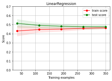
../_images/NOTES 05.02 - MODEL EVALUATION_41_0.png

Diagnosing¶

Linear regression BASELINE

estimator = LinearRegression()
cv = ShuffleSplit(n_splits=10, test_size=.3)
ch.plot_learning_curve(estimator, estimator.__class__.__name__, X, y, cv=cv, scoring=rel_mrae, ylim=(0,0.7))

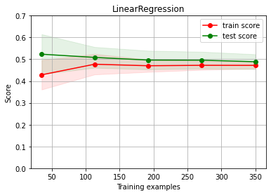
../_images/NOTES 05.02 - MODEL EVALUATION_43_0.png

We have UNDERFITTING (high bias)

increase model complexity
get more columns

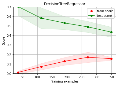
# try first increasing model complexity --> a bit better but with overfitting
# experiment with different max_depth values

from sklearn.tree import DecisionTreeRegressor
estimator = DecisionTreeRegressor(max_depth=8)
ch.plot_learning_curve(estimator, estimator.__class__.__name__, X, y, cv=cv, scoring=rel_mrae, ylim=(0,0.7))

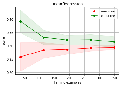
../_images/NOTES 05.02 - MODEL EVALUATION_45_0.png

# try now with more columns (we have them!!!) --> improves a bit

d2 = pd.read_csv("local/data/cal_housing_small_full.data")
d2.head()

	longitude	latitude	housingMedianAge	totalRooms	totalBedrooms	medianHouseValue	population	households	medianIncome
0	-120.58	35.00	37.0	523.0	119.0	106300.0	374.0	95.0	1.4726
1	-118.17	33.98	31.0	1236.0	329.0	155400.0	1486.0	337.0	3.0938
2	-122.22	37.81	52.0	1971.0	335.0	273700.0	765.0	308.0	6.5217
3	-117.91	33.66	21.0	1708.0	505.0	193800.0	1099.0	434.0	3.2250
4	-121.92	37.24	27.0	1265.0	216.0	281200.0	660.0	232.0	5.3911

estimator = LinearRegression()
X2 = d2[[col for col in d2.columns if col!="medianHouseValue"]].values
y2 = d2["medianHouseValue"].values
print (X2.shape, y2.shape)

ch.plot_learning_curve(estimator, estimator.__class__.__name__, X2, y2, cv=cv, scoring=rel_mrae)

(500, 8) (500,)

Diagnosing¶

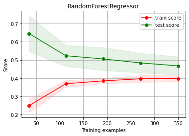
Random Forest BASELINE

from sklearn.ensemble import RandomForestRegressor
estimator = RandomForestRegressor(max_depth=10)
(trmean, trstd), (tsmean, tsstd) = bootstrap_score(estimator, X, y, test_size=0.3)
print ("train score %.3f (±%.4f)"%(trmean, trstd))
print ("test score  %.3f (±%.4f)"%(tsmean, tsstd))

train score 0.158 (±0.0078)
test score  0.362 (±0.0226)

../_images/NOTES 05.02 - MODEL EVALUATION_49_1.png

ch.plot_learning_curve(estimator, estimator.__class__.__name__, X, y, cv=cv, scoring=rel_mrae)

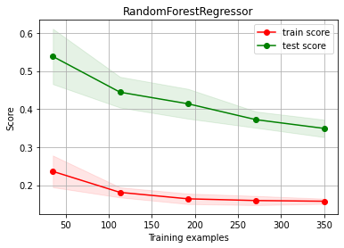
../_images/NOTES 05.02 - MODEL EVALUATION_50_0.png

We have OVERFITTING (high variance)

reduce model complexity
get more data

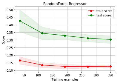
# try first reduce model complexity --> more BIAS
estimator = RandomForestRegressor(max_depth=4)
ch.plot_learning_curve(estimator, estimator.__class__.__name__, X, y, cv=cv, scoring=rel_mrae)

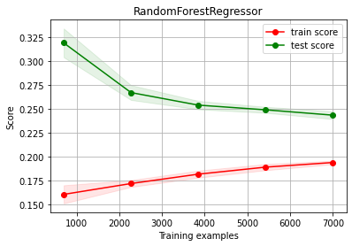
../_images/NOTES 05.02 - MODEL EVALUATION_52_0.png

# try now with more data (we have A LOT!!!) 

d3 = pd.read_csv("local/data/cal_housing.data")
print ("TOTAL AVAILABLE DATA", d3.shape)
d3 = d3.sample(10000)
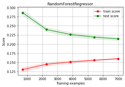
estimator = RandomForestRegressor(max_depth=10)
X3 = d3.values[:,:-1]
y3 = d3["medianHouseValue"].values
print ("building learning curve with", X3.shape, y3.shape)

ch.plot_learning_curve(estimator, estimator.__class__.__name__, X3, y3, cv=cv, scoring=rel_mrae)

TOTAL AVAILABLE DATA (20640, 6)
building learning curve with (10000, 5) (10000,)

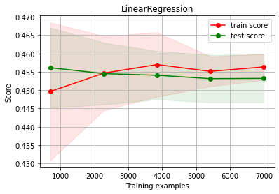
../_images/NOTES 05.02 - MODEL EVALUATION_53_1.png

What if we made the wrong choice¶

Linear Regression UNDERFITTING and choose acquire more data: No improvement!!!

estimator = LinearRegression()
ch.plot_learning_curve(estimator, estimator.__class__.__name__, X3, y3, cv=cv, scoring=rel_mrae)

../_images/NOTES 05.02 - MODEL EVALUATION_55_0.png

Random Forest OVERFITTING and choose to add more columns: some improvement!!!

estimator = RandomForestRegressor(max_depth=10)
ch.plot_learning_curve(estimator, estimator.__class__.__name__, X2, y2, cv=cv, scoring=rel_mrae)

../_images/NOTES 05.02 - MODEL EVALUATION_57_0.png

let’s now choose more data and more columns (a luxury!!!)

d4 = pd.read_csv("local/data/cal_housing_full.data")
print ("TOTAL AVAILABLE DATA", d4.shape)
d4 = d4.sample(10000)
estimator = RandomForestRegressor(max_depth=10)
X4 = d4.values[:,:-1]
y4 = d4["medianHouseValue"].values
print ("building learning curve with", X4.shape, y4.shape)

ch.plot_learning_curve(estimator, estimator.__class__.__name__, X4, y4, cv=cv, scoring=rel_mrae)

TOTAL AVAILABLE DATA (20640, 9)
building learning curve with (10000, 8) (10000,)

../_images/NOTES 05.02 - MODEL EVALUATION_59_1.png

Inteligencia Artificial para las Ciencias e Ingenierías

05.02 - MODEL EVALUATION

Contents

05.02 - MODEL EVALUATION¶

See my courses and progress

The `cal_housing` repository publicly available¶

Understand data¶

Show house locations on map¶

Separate variable to predict¶

A linear regression¶

How sure can we be of our model performance¶

Diagnosing¶

Diagnosing¶

What if we made the wrong choice¶

Inteligencia Artificial para las Ciencias e Ingenierías

05.02 - MODEL EVALUATION

Contents

05.02 - MODEL EVALUATION¶

See my courses and progress

The cal_housing repository publicly available¶

Understand data¶

Show house locations on map¶

Separate variable to predict¶

A linear regression¶

How sure can we be of our model performance¶

Diagnosing¶

Diagnosing¶

What if we made the wrong choice¶

The `cal_housing` repository publicly available¶